Atlas: Orienting the Pre-Training data of an LLM

The Concept Atlas below is an interactive visualization (UMAP projection) showcasing a representative 10% subset (3,372 concepts) from our comprehensive set of 33,732 concepts.

Loading visualization...

Shown below are two examples: one about a text related to Mythology and another one on Orbital Mechanics. We demonstrate how Atlas maps the tags associated with each text to human-interpretable concepts and descriptions within the concept library.

Introduction

At Guide Labs, we are building models whose reasoning and representations are transparent, so that humans can audit and understand them. Achieving this goal requires that a model’s internal representations align with concepts: coherent and atomic human-meaningful units, rather than inscrutable statistical features and correlations. We set out to pre-train language models on large-scale corpora in a way that constrains the model’s internal representations to be cleanly decomposable into these concepts. Consequently, we needed a comprehensive concept library for contemporary LLM pre-training corpora.

Goals. With this vision in mind, we set out to build a concept library suitable for supervising large-scale LLMs during pre-training, mid-training, and post-training. Such a library must be:

• Multi-scale: covering both high-level themes and fine-grained units.
• Stylistically expressive: capturing attributes like tone or formality, not just semantic categories.
• Localizable: applicable to spans within a document, enabling sub-document-level control and edits.
• Human-meaningful: comprising concepts that people actually care about understanding and controlling.
• Representative: spanning broadly enough to cover the true distribution of large-scale LLM pre-training corpora across webtext, code, math, and scientific writing.

No human-interpretable concept library for LLM pre-training data existed at scale

Before building our concept library, we surveyed existing approaches in the language modeling literature for large-scale concept extraction. We found no concept library that was both human-interpretable and representative of real pre-training data at scale. Broadly, concept libraries fall into three categories.

Word-based concept dictionaries. For example, Luo et al. construct a 40,000-item concept dictionary by selecting the most frequent words from the Brown Corpus and prompting GPT-4 to generate sentences illustrating each word. However, single words cannot capture the higher-level abstractions, multi-sentence topics, or domain-specific ideas that appear throughout pre-training corpora.

Activation-derived, unsupervised concepts. Other works extract concepts directly from model activations, such as directions discovered via sparse autoencoders (SAE). It has become doubtful whether these concepts reflect the model’s internal structure. Further, SAE-derived concepts are not necessarily human-meaningful.

Narrow-domain supervised libraries. Some concept sets focus on specific tasks such as sentiment or toxicity. These offer high-quality labels but are too narrow to supervise models trained on diverse corpora spanning webtext, code, math, and scientific writing.

Our contribution. In the rest of this post, we describe how we built a concept library with over 33,000 concepts, covering webtext, code, mathematical content, and scientific topics. We begin with an overview of the datasets we have annotated, then walk through our annotation pipeline. Finally, we show how Atlas enables the deduplication of millions of raw, freeform annotations into a canonical set of coherent, human-meaningful concepts suitable for supervising LLMs.

Methods

To develop models whose internal representations can be aligned with human-interpretable concepts, we first needed a concept-annotated pre-training corpus large enough to reflect the full conceptual breadth of modern LLM datasets.

We began by constructing a representative sample of our pre-training and mid-training data mixtures. This sample spans: webtext, code, math, scientific writing, encyclopedic content, question–answer exchanges, and instruction-following data. In total, we collected 6.6 million documents, balanced across six major document categories(roughly one million documents per each), including:

• Webtext: DCLM (deduplicated),
• General academic knowledge: Pes2o, Arxiv, Wikipedia and Wikibooks
• Math: Dolmino-math, including GSM8K
• Code: StarCoder
• Q&A: FLAN v2

DCLM is a high-quality dataset that uses model-based quality filtering to filter a large subset of the Common Crawl for similarity to OpenHermes and other instruction-tuning datasets. DCLM contained a large fraction of duplicates (approximately 80% duplicated content). Therefore, we used the deduplicated version of DCLM from Zyda-2. Our pre-training and mid-training data mixture follows the Olmo recipe with some notable exception.

These documents vary substantially in style, purpose, and conceptual density, making them an ideal substrate for large-scale concept extraction. From these documents we generated 44 million text chunks, each representing a short semantically coherent span (typically 128–256 tokens depending on the domain). These chunks form the fundamental units we annotate. Aggregated over all domains, our annotation pipeline produced nearly 500 million tags, of which 14 million were unique tags and 1 million appeared more than 15 times. This large, diverse, and redundant tag space is essential for the clustering and canonicalization procedures that follow.

Evaluation Procedure: LLM Concept Validation

Across all stages of the pipeline, we rely on a unified evaluation framework to measure annotation quality, concept coherence, and classifier performance. Each annotation, whether a raw tag, a canonicalized concept, or a predicted label from the final concept annotator model, is scored by human raters and LLM judges on a 1–5 scale. We designed the benchmark such that a score of 2 or higher is considered successful, i.e, the concept is minimally present. This threshold is intentionally permissive: minor tags capture fine-grained contextual details. We visualize these scores using per-tag and per-chunk histograms.

This evaluation method appears repeatedly throughout the rest of the post, as we assess:

• the recall and relevance of raw tags (Stage 1),
• the coherence and redundancy of concept clusters (Stage 2), and
• the accuracy and calibration of predictions from the final concept annotator model (Stage 3).

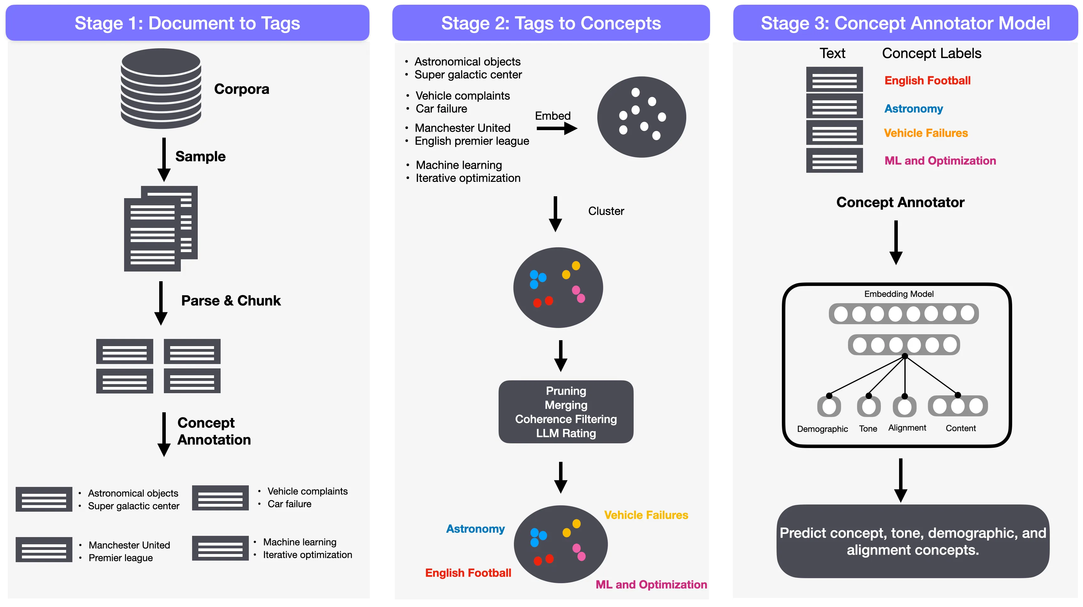
Stage 1: Documents → Tags

In this stage, we seek to convert raw documents into structured semantic tags that describe the key concepts present in them. These raw tags are intentionally allowed to be broad, granular, and overlapping; hence, they serve as the raw material from which we will later derive a canonical concept library. For this stage, the priority is coverage rather than precision: we want as many concept candidates as possible, across all domains and levels of granularity.

At a high level, Stage 1 consists of three operations:

• splitting documents into chunk-sized spans,
• prompting a model to generate structured annotations for each span, and
• validating these annotations using the global scoring methodology described in the overview section.

The remainder of this section details the engineering decisions behind each step and the empirical results that demonstrate the success of Stage 1.

Chunking: Converting Documents into Chunk-Level Annotation Units

LLMs often do not annotate whole documents well: long documents contain multiple unrelated concepts, and annotation models tend to default to high-level summaries rather than the granular conceptual units. We therefore annotate at the chunk level, typically capturing one coherent idea, argument, problem, or algorithmic structure. A chunk is a short, semantically coherent segment of text, typically 128–256 tokens, created by concatenating consecutive sentences until a domain-specific token limit is reached. Chunks are the fundamental units of annotation in Stage 1: every chunk receives a structured set of tags describing its conceptual content.

We perform high-speed chunking by first detecting sentence boundaries using blingfire, then tokenizing and concatenating sentences until a domain-specific threshold is reached: 150 tokens for webtext and general documents, 256 tokens for math and code, where a single idea requires more context. Sentences which exceed the threshold are treated as single chunks, unless they exceed 50,000 tokens (in which case they are dropped). This adaptive thresholding ensures that each chunk contains a complete semantic unit rather than arbitrary fragments.

This process yielded 44 million chunks from 6.6 million documents. Chunking at this granularity proved essential: concept labels applied at the chunk level map closely to local meaning, enabling fine-grained conceptual decomposition. Click through the panels below to see real examples of how documents are chunked across different domains.

WebTextWikipediaMathCode

Structured Annotation Schemas: Domain-Aware Tagging

Different domains express conceptual structure differently. A Wikipedia article, a math proof, a stack exchange Q&A, and a block of Python code demand different concept ontologies. We therefore extracted domain-specific structured tag schemas, each containing 4–6 domains or fields tailored to the content type. Each field expands into a hierarchical tag, from broad to narrow and granular, and together they produce on average 10–15 tags per text chunk. These chunk-extracted tags form the basis for Stage-2 of our Atlas pipeline.

The examples above illustrate the consistency and richness of the structured fields: each annotation combines topic, purpose, structure, and secondary concepts, generating a high-recall conceptual snapshot of each chunk.

Annotator Model Selection

We evaluated several open-weight models for annotation. While the Phi models could output consistently structured annotations, they suffered from repetition and frequent collapse into degenerate loops, making it unusable for long-running annotation. Qwen 2.5 7B performed better semantically but more unpredictably syntactically, often producing the wrong number of fields and generating responses that were difficult to parse reliably. In contrast, Mistral small 3.1 (a 24B model) consistently adhered to the structured format, avoided repetition collapse, and maintained stable behavior across millions of prompts. In the end, Mistral was the smallest model that satisfied our formatting and reliability constraints; even a 1% schema deviation across 44 million chunks would produce nearly half a million unusable annotations, so predictability was essential.

Output of Stage 1: A High-Recall Pool of Raw Tags

Stage 1 produced:

• 44 million annotated chunks
• 500 million short tags extracted from structured fields
• 14 million unique short tags after deduplication
• 1 million short tags with >15 occurrences

This raw tag space is intentionally redundant and noisy. The purpose of Stage 1 is not to produce the final concept inventory; it is to cast a wide semantic net. The refinement and consolidation into 33,000 canonical concepts happens in Stage 2.

Using the global scoring framework introduced earlier, where both humans and LLM judges rate each tag and chunk on a 1–5 scale, we evaluated the output of Stage 1. A score of 2 or higher counts as successful, reflecting both the high-recall objective of this stage and the inherent granularity of minor tags. Across all domains, almost every tag scored at least a 2, and chunk-level averages are between 3.5 and 4.2. Human audits confirmed that the tags were conceptually relevant and coherent.

Stage 2: Tags → Concepts

Stage 2 transforms millions of noisy, free-form tags into a coherent library of more than 33,000 human-interpretable concepts. Through large-scale embedding, clustering, LLM-based cluster coherence evaluation, concept labeling, and graph-based deduplication, we create a diverse and comprehensive concept inventory that reflects the true semantic structure of our data corpus.

Tag Normalization and Embedding

The first challenge is that short-tags generated in Stage 1 are highly variable. Minor formatting differences, hyphens, slashes, whitespace, punctuation artifacts, can split semantically identical tags into separate strings. Before clustering, we normalize all tags into a standardized form, with examples shown below.

Raw Tag	Normalized Tag
astronomical-objects	astronomical objects
climate-change \n adaptation	climate change adaptation
machine-learning / ai	machine learning ai

Top-100 Most Frequent Tags

academic writingresearch reportingscience researchbiologyphysicsmathematicscomputer sciencemedicinedata analysismolecular biologytechnologyresearch methodologyexperimental resultsscientific explanationchemistrystatisticsreal world contexttheoretical physicsmachine learningarithmeticeducationalalgorithmscomputationeducationmathematical conceptsastrophysicsnotationanalysisfictionprogrammingtechnical explanationacademic discussiongeneticsinformationalsoftware developmentequationsdocumentationengineeringcomparisoninformation sharingmethodologycommunicationnarrativematerials sciencefunctionsgeographycomparative analysisresearch methodssource codeeconomics

Show 50 more tags

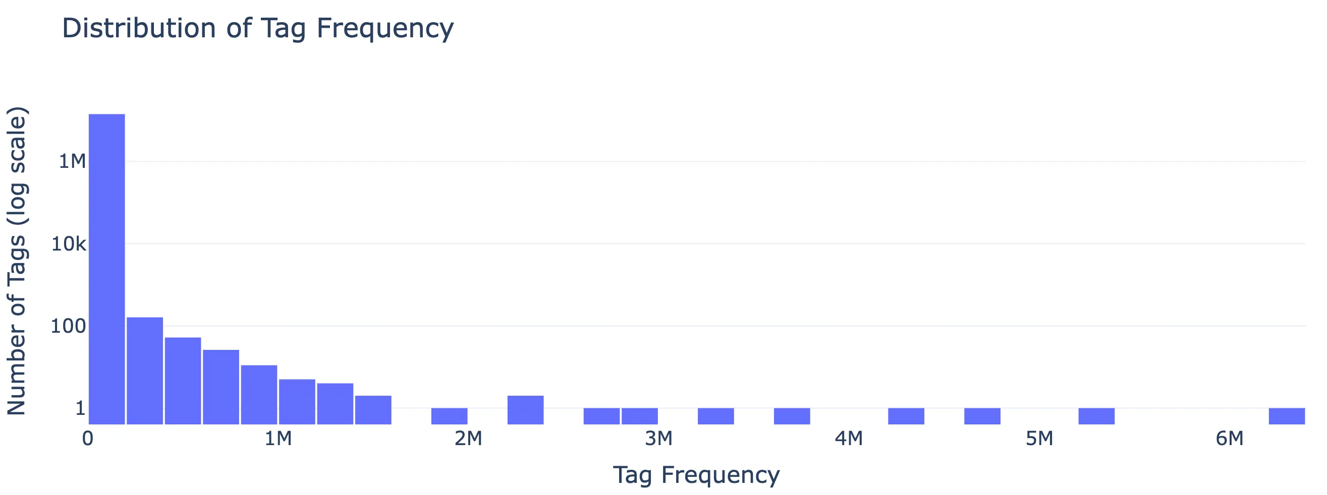
After standardizing and deduplicating raw tags, we obtain nearly 14 million unique normalized tags for semantic modeling. Most tags appear very infrequently (less than 5 times), whereas tags that appear more than 10 times constitute only about 10% of the total as shown in the tag distribution plot above.

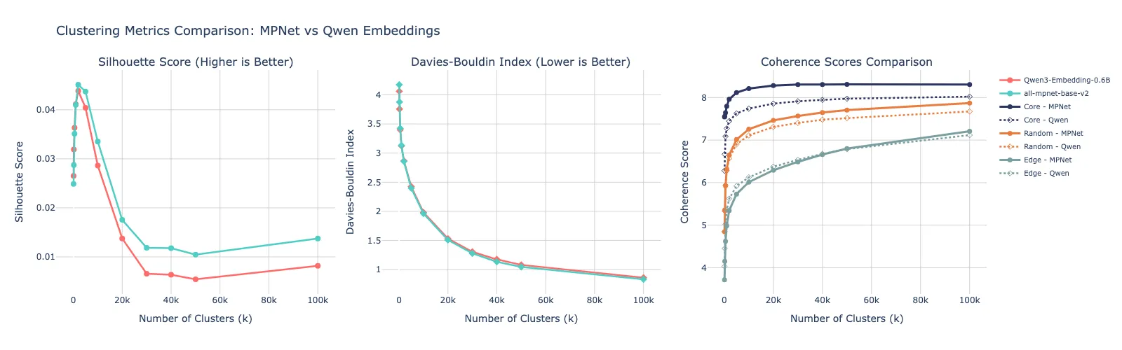
To capture the meaning of each tag, we used the all-mpnet-base-v2 embedding model to embed and convert them into 768-dimensional vectors. These vectors are dense, numerical representations that encode the semantic similarity between tags in a high-dimensional space. We experimented with other embedding models, such as Qwen3-Embedding-0.6B, but all-mpnet-base-v2 produced slightly better-quality clusters, confirmed by standard metrics like the Silhouette score and Davies–Bouldin index (discussed below). This embedding step produces 14 million vectors, one for every unique tag, capturing the conceptual hint extracted from the original text chunks.

Clustering Tags into Semantic Groups

With all tags embedded in a common vector space, we cluster them into groups representing potential concepts. The goal is to group tags that are semantically similar, e.g., “frozen planet,” “icy satellites,” and “interstellar ice diffusion” into the same conceptual region or cluster. We use the K-Means algorithm to cluster tag embeddings, implemented efficiently using the FAISS library, chosen for its efficiency and ability to handle tens of millions of vectors on GPU. K-Means is an iterative algorithm that determines a set of K cluster centers (centroids) by minimizing the following objective function, also known as the Within-Cluster Sum of Squares (WCSS). In our implementation, each tag embedding is assigned to the nearest centroid by maximizing the cosine similarity metric (which is mathematically related to minimizing L2 distance on normalized vectors).

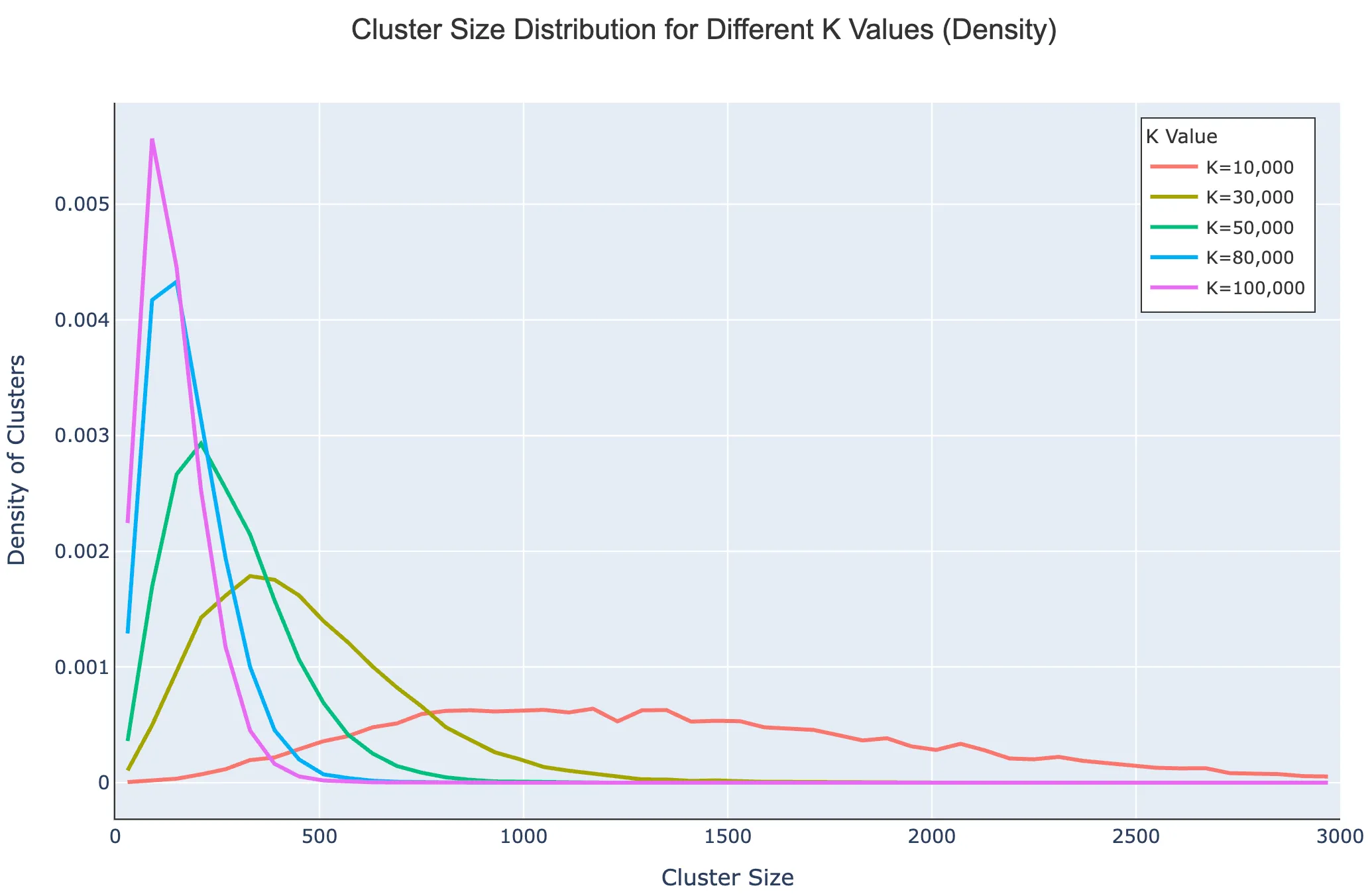
Because the number of true underlying concepts is unknown, we sweep over a wide range of cluster sizes: k ∈ {100, 500, 1k, 10k, 20k, 30k, 50k, 80k, 100k}. Small k values (fewer clusters) result in very large, diverse clusters that contain a wide variety of tags. Large k values (many clusters) naturally create tighter, more specific clusters, but this risks fragmenting genuinely related concepts or introducing clusters based on noise. We evaluate the quality of each k value using multiple metrics to select the near-optimal number of clusters:

1. Silhouette Score: Measures how similar each point is to its own cluster compared to other clusters (higher is better, range -1 to 1).
2. Davies-Bouldin Index: Measures the average ratio of within-cluster distances to between-cluster distances (lower is better).
3. LLM-based Coherence Scoring: A subjective measure of the semantic quality and cohesiveness of the tags within each cluster (higher is better)

The Silhouette score peaks early and then decreases with k, while the Davies–Bouldin index decreases monotonically. Since we compute these metrics on a sub-sample of the 14 million points, they don’t accurately represent cluster quality at different k values. We therefore rely on LLM-based coherence evaluation.

We perform a semantic coherence evaluation on every cluster. This is necessary because not all K-Means clusters represent genuinely meaningful concepts—some may be artifacts of the embedding process or lexical coincidences. For each cluster, we sample three strata of tags: Core tags (closest to centroid), Random tags (uniform sample), and Edge tags (farthest from centroid). We group tags into sets of 10 and query an LLM (Mistral-Small-3.1-24B) to score coherence on a 1–10 scale.

Coherence improves steadily as k increases, plateauing around k = 60,000 – 80,000. Beyond this range, computational cost rises while semantic gains diminish. We select k = 80,000, producing clusters that balance granularity, separation, and interpretability. Most clusters contain 200–500 tags, though sizes vary depending on domain density and tag frequency.

We retain only high-quality clusters that meet minimum coherence thresholds: core coherence ≥ 9, random coherence ≥ 8, and edge coherence ≥ 7. These thresholds ensure clusters are conceptually tight at their centers and maintain semantic coherence at their edges. Of the initial 80,000 clusters, 17,443 failed our criteria and were removed, leaving 62,557 high-quality semantic units. This step substantially improves the signal-to-noise ratio and prepares clusters for labeling into human-understandable concepts.

Cluster Labeling and Deduplication: Producing Human-Readable Concepts

With a high-quality set of clusters, we convert each one into a readable, human-interpretable concept. Each concept receives a 1–6 word label and a concise, descriptive sentence explaining its meaning. For each cluster, we sample 50–100 representative tags (weighted by frequency) and use a 24B Mistral model to generate a concise label and a one-sentence description. These labels provide a clean, human-friendly interpretation of dense semantic clusters. We then embed the LLM-generated concept names and descriptions using a Qwen3-Embedding-0.6B instruction-tuned embedding model, producing a semantic space of concepts.

The interactive visualization below shows the embedding space of tags colored by their assigned clusters. Each point represents a tag, positioned according to its semantic similarity to other tags. Hovering over points reveals the tag text, its cluster assignment, and the mean coherence score of its cluster. The visualization also highlights several low-coherence clusters that were filtered out by our coherence thresholds, demonstrating how quality control removes semantically inconsistent groupings.

Loading visualization...

The concept embeddings in 1024-dimensional space reveal significant duplication based on name and description similarity. This makes merging similar concepts necessary. The challenge is determining which concepts to merge and at what granularity. We address this through an iterative graph-based merge discovery and concept merging process.

Concept Deduplication: For each concept, we embed it using the qwen3-embedding-0.6B model with its name and description. We then find its Top-20 nearest neighbors based on cosine similarity and retain neighbors with similarity above 0.85. Next, we construct an undirected similarity graph where nodes are concepts and edges connect nodes whose cosine similarity meets the threshold. We run the Louvain community detection algorithm to identify groups of related concepts. Each connected component represents a candidate merge set. For each potential merge set, we checked the groups and combine member concepts by regenerating a label and concise rich description using an LLM. This process reduces the count to around 39,000 concepts. We repeat merging for 2–3 iterations until reaching 35,000 concepts with acceptable diversity among the most similar concepts.

Evaluation

To evaluate the quality of the final canonical concepts and their suitability for downstream annotator training, we applied the same human + LLM scoring framework introduced earlier. We sampled concepts and the chunks associated with them, scoring both the concept labels and the chunk–concept assignments on the 1–5 scale used throughout this work. Concept-level evaluation shows that the vast majority of concept labels score between 3.5 and 4.5, with only a small tail below 3—indicating that the labeling and deduplication pipeline consistently produces clear, human-interpretable concepts. When we evaluate chunk–concept alignment, we achieve a ~97% success rate (score ≥ 2) across the 2.3 million chunks used as training data for content concepts. This high alignment rate confirms that the clusters are not only semantically coherent internally but also accurately represent the conceptual content present in real text.

Final Concept Library

This process reduces 62,557 coherent clusters to 33,000 final canonical concepts.These final concepts represent distinct, interpretable elements of the conceptual landscape of our corpus. Some conceptual overlap and hierarchy is inevitable, real-world knowledge is not cleanly partitioned, but the deduplicated set strikes a practical balance between granularity and clarity.

Concept Taxonomy

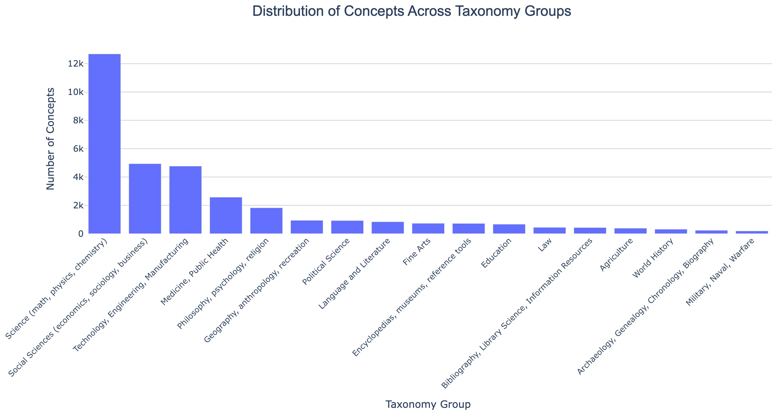
We organized our 14 million unique concept tags into a hierarchical taxonomy based on the Library of Congress classification system, mapping our concepts to approximately 2,600 nodes across a tree structure with 20 top-level branches and ~6,500 total nodes (with depth up to 9 levels). Below, we show a distribution of concepts across these taxonomy groups. Science (Q) dominates with 38% of concepts, followed by Technology (T) at 15%, Social Sciences (H) at 15%, and Medicine (R) at 8%, with all 20 root branches represented to varying degrees.

Within the heavily-populated Science branch, mathematics and physics subcategories are particularly prominent, QA (Mathematics) subdivisions like Analysis (QA299.6-433), Geometry (QA440-699), and Algebra (QA150-272.5) account for over 3,700 concepts combined, while QC (Physics) areas like Atomic/Molecular Physics (QC170-197) contribute another 662 concepts, alongside substantial representation in Technology areas like Telecommunications (TK5101-6720) and Computer Hardware (TK7885-7895).

This taxonomy provides a structured framework for understanding the topical coverage of our training data and enables hierarchical analysis of concept distributions across different knowledge domains.

This canonical concept library serves as the foundation for Stage 3, where we train a concept annotator model capable of labeling arbitrary text with these concepts.

Stage 3: Concept Annotator Model

The final stage of the pipeline is to train a model that can assign concepts directly to text. Whereas Stage 1 produced raw chunk-level tags and Stage 2 distilled them into a canonical library of ~33,000 coherent concepts, Stage 3 builds a model capable of recognizing these concepts in arbitrary text. This model, the multi-domain, multi-label concept annotator, is what ultimately enables concept-supervised pre-training across the entire pre-training corpus, including concept-aware fine-tuning.

We aim to predict concepts across four distinct taxonomies: content, tone, demographic, and alignment. Each category has different structures, and label counts. Rather than maintain four separate classifiers (with separate encoders, heads, thresholds, and inference logic), we train a single unified model that jointly predicts all four domains while sharing computation, embeddings, and inference pipelines.

Goals and Design Principles

Three design constraints shaped the annotator architecture:

• One model, multiple domains: Maintaining four different classifiers would complicate the training and inference stack. A single model with separate output heads keeps the system simple and maintainable.
• Incorporate the strengths of the KNN baseline: A simple KNN classifier over Stage 2’s concept embeddings performs surprisingly well on content-label prediction, especially for frequent, well-represented concepts. The question was whether a learned model could surpass similarity-based retrieval while retaining its strengths.
• Positive-Unlabeled (PU) supervision: The data contains only positive labels for each domain: no negative annotations. This requires careful definition of target spaces, loss functions, and evaluation metrics. These constraints drove the design of a multi-head MLP on top of a shared encoder.

Supervision: Positive–Unlabeled Learning

Because each chunk is labeled only with the concepts it should have, never with the concepts it explicitly should not have, supervision follows a Positive and Unlabeled (PU) paradigm.

Each concept receives one of three labels: +1 — positive, 0 — unlabeled, –1 — explicit negative (rare; used only after optional negative sampling). During training, we optionally sample a small number of synthetic negatives per example to stabilize learning. PU learning influences both training (via masked-BCE and PU loss) and metrics (via PU-aware scoring callbacks)

Input Representation and Targets

Atlas tokenizes text using Qwen3-Embedding-0.6B and maps each example to a concept vector via CLS or last-hidden-state pooling. To prevent rare concepts from being drowned out, it uses a rarity-weighted sampling scheme that boosts underrepresented labels during training; critical for stable learning on long-tail distributions.

Model Architecture and Encoder

The annotator is a Qwen-based encoder with a shared trunk and domain-specific heads. A Qwen3-Embedding-0.6B model produces a pooled embedding for the input text. This embedding flows into: A lightweight MLP with: LayerNorm, ReLU, Dropout and Projection back to 1024 dimensions. This trunk supports the tone, demographic, and alignment heads, while content labels follow a slightly different path.

Content Head: Dot-Product with Label Embeddings

Content concepts are embedded into a label matrix, with predictions made directly from encoder output; bypassing the shared MLP trunk to preserve KNN-like signal while still allowing learned improvements. Tone, demographic, and alignment heads use simpler linear classifiers, which suffice for their lower-cardinality domains.

Losses

We combined two loss functions: Masked Binary Cross-Entropy (Standard BCE applied only to the positions where targets are non-zero), and Non-negative PU Loss. A PU-compatible objective penalizes overconfident positives on unlabeled classes and stabilizes long-tail learning. This combination handles both positive-only supervision and the occasional sampled negative.

Evaluation Metrics

We tracked metrics such as Precision-Recall Metrics, Macro Average Precision (PR-AUC) per domain, Precision@5, and Recall@10. However, principal reliance on them is problematic for PU (positive-unlabeled) learning because without confirmed negatives, any unlabeled example predicted as positive gets counted as a false positive; even if it’s actually correct. This systematically deflates precision and PR-AUC, making model performance appear worse than it is. The metrics still track relative improvement across runs, but absolute values should be interpreted with caution. Consequently, we rely mostly on the LLM Concept Validation procedure we discussed earlier.

Using the global scoring framework from earlier stages, we evaluate how well the annotator’s predictions align with human assessments. Across 2.3 million chunks used in annotator training, we achieve a ~97% success rate (score ≥ 2) when comparing predicted concepts with human ratings. Score distributions cluster strongly between 3.5 and 4.3, indicating that the model consistently assigns coherent, meaningful concepts to text across all domains. This confirms that Stage 3 successfully operationalizes the canonical concept library derived in Stage 2.

Conclusion

We have presented Atlas, a 3 stage pipeline, for concept annotation of large-scale LLM pre-training corpora. By moving from raw documents to high-recall chunk tags to coherent canonical concepts to a unified multi-domain annotator, we create a foundation that enables interpretable model training. While there is still room for refinement, the combination of large-scale automation and targeted human validation proves that high-quality concept structure can be embedded directly into modern LLM workflows.