We have developed a new type of discrete diffusion language model that replaces traditional full attention with block causal attention. We scaled this architecture to billions of parameters and observed that the model generates coherent text without incurring downstream performance trade-offs on benchmarks, compared to standard diffusion alternatives.
Causal Diffusion Language Models

Authors: Aya Ismail, Co-Founder & CSOJulius Adebayo, Co-Founder & CEO
Published: December 04, 2025
Below, we show samples generated from a 1.5 billion parameter causal diffusion language model (CDLM) trained on 150 billion tokens from the Nemontron-cc-hq corpus.
Loading generation examples...
Introduction
Contemporary language models fall into two broad families: Autoregressive models (AR) and Diffusion language models (DLMs). AR models, GPT style, learn to extend a prefix by predicting the next token, whereas discrete diffusion models learn to reconstruct tokens at all positions from corrupted versions of the input.
This difference in training objectives leads to distinct sampling dynamics and trade-offs in interpretability, controllability, and scaling properties. AR models produce a long chain of single-token completions, whereas diffusion models expose joint, multi-token updates, which is attractive for settings where steering and interpretability are critical.
In this post, we:
- Provide an overview of AR (GPT-style) and standard discrete diffusion language models. We highlight specific aspects of each model class that hinder interpretability, our principal requirement.
- Introduce Causal Diffusion, a diffusion language model variant that incorporates a block-causal attention structure.
- Demonstrate empirically that CDLMs outperform standard diffusion models across a variety of benchmarks and compare favorably with their autoregressive counterparts.
Motivation
At Guide Labs, we are building models whose internal representations can be explained and steered in terms of topics and concepts that a human can easily understand. Our approach is to constrain the model’s representations during training to encode these human-understandable concepts directly. For any group of output tokens, we would like to trace their generation to specific concepts that are causally responsible for their generation.
First, let us define a concept as a coherent, atomic, human-meaningful unit. Concepts induce a distribution over the vocabulary of a model. Concepts rarely reduce to a single token. Instead, a concept induces a distribution over many tokens. For example, a document about economics is more likely to contain words such as supply, demand, trade, and bank. A document about machine learning emphasizes neural networks, optimization, and models. Abstract behavioral concepts like politeness, regret, apology, and sarcasm manifest across phrases and clauses, not isolated tokens.
Simultaneously explaining and steering a model’s output using concepts requires tight coupling between the model’s output and the concepts. This is fundamentally challenging for autoregressive models: while these models can compute losses over multiple tokens, their underlying autoregressive factorization still prioritizes single-token decisions. As a result, multi-token concepts are not easily expressed or controlled as coherent units. Moreover, while AR models can generate long sequences, the next-token objective limits concept-level controllability over extended contexts. In contrast, diffusion models update many token positions jointly at each denoising step, providing a natural mechanism for concept-level steering.
Because these concepts span multiple tokens, models that expose joint, multi-token update steps provide a more natural interface for concept-level control. Diffusion models meet this requirement: at each unmasking step, they update many positions simultaneously, allowing concept-level interventions that propagate in a coherent and interpretable way.
Overview of Language Model classes
At a high level, a language model processes a sequence and determines how each position should be updated. One main difference between AR and diffusion LMs is in the dependency allowed between tokens, as defined by the attention mask. For instance, given the sequence ‘The cat sat on the’, an autoregressive model restricts each token to attend only to earlier tokens, while a diffusion model permits every token to draw on context from the entire sequence. We will illustrate here how we relax such restrictions and arrive at a diffusion LM with a new attention structure.
Autoregressive Language Models
These are by far the most popular type of LLMs. Most frontier systems live in this family. Autoregressive (AR) models are trained to predict the next token given the previous ones, so they’re often referred to as next-token predictors. Concretely, they use a transformer with a causal attention mask that lets each token attend only to earlier tokens.
Pros: Excellent empirical scaling, lots of engineering experience, very strong performance across domains.
Cons: The model generates one token at a time, which makes it less natural to control properties that are expressed over multi-token spans.
Diffusion Language Models
Diffusion language models take almost the opposite approach. They are often referred to as any-order models: they’re trained with a bidirectional attention mask, randomly masking tokens and learning to predict the masked ones.
Recently, Nie et al. (2025) successfully trained the first large diffusion language model (LLaDA) from scratch, achieving performance competitive with state-of-the-art open-source AR models. Since then, several commercial DLMs have emerged, showing very low generation latency due to parallel decoding, including Mercury, Gemini-diffusion and Seed Diffusion.
Pros: Any-order modeling is naturally suited to tasks with non-causal dependencies, and multi-token generation is built in, so inference can be very fast. It also aligns well with scenarios where we ultimately want to control behaviour over multi-token spans.
Cons: For a fixed compute budget, their scaling is noticeably weaker than AR models. They’re also quite new, so the “right” architectures and training tricks are still being figured out.
From Diffusion to Blockwise Diffusion
Standard diffusion LMs like LLaDa train with full attention and random masking patterns, but often generate with a semi-autoregressive schedule: the sequence is split into blocks, and at each step the model denoises one block before moving to the next.
This leads to a train/inference mismatch. During training, every token can in principle see every other token with random masking patterns. But during inference, tokens in a block can only see the current partially denoised block and past blocks, while future blocks are completely masked.
Block Diffusion LMs were introduced to fix this mismatch. They use a block-causal attention mask that is bidirectional within a block but causal across blocks, and they train on a concatenation of a noisy half and a clean half of the sequence.
The intuition is straightforward: the noisy half learns to denoise the current block, while the clean half provides the already-denoised history of previous blocks. This approach removes the train/inference mismatch, but comes with a significant cost. The sequence is effectively duplicated, with half the context wasted on carrying clean copies of tokens that also appear in the noisy half. This makes Block Diffusion models roughly 2× more expensive to train than comparable DLMs with the same context window.
Causal Diffusion
The main issue with Block Diffusion is its 2× training cost due to the clean half duplication, so one obvious question is: Do we really need the clean half? Our answer is no. We found we can keep the nice semi-autoregressive structure of Block Diffusion while dropping the clean half entirely. We call the resulting models Causal Diffusion Language Models.
At a high level, a Causal Diffusion LM has:
- A single noisy sequence: We do not concatenate noisy + clean; we diffuse over one sequence
- Block-causal attention: Within a block: full bidirectional attention. Across blocks: causal, where a block can only attend to previous blocks and itself, never future blocks
- Per-block noise schedules: Different blocks in the same sequence can be at different noise levels, but they all live in the same stream of tokens
Compared to other approaches, Causal Diffusion offers distinct advantages. Versus autoregressive models, we still have a causal structure across blocks but can update whole blocks of tokens at once. Versus standard diffusion LMs, we keep denoising-style training but no longer rely on full attention. Versus Block Diffusion, we keep the block-causal structure but drop the clean half and its 2× context overhead.
This blockwise structure isn’t just a decoding trick. Many attributes we ultimately care about, tone, formality, hedging, whether a passage expresses regret or apology, are usually expressed over multiple tokens at once. Having an architecture that naturally reasons at the block level, rather than only one token at a time, will be important later when we start thinking about controlling these higher-level properties.
To illustrate these different attention patterns, here’s a side-by-side comparison of all the approaches we’ve discussed:
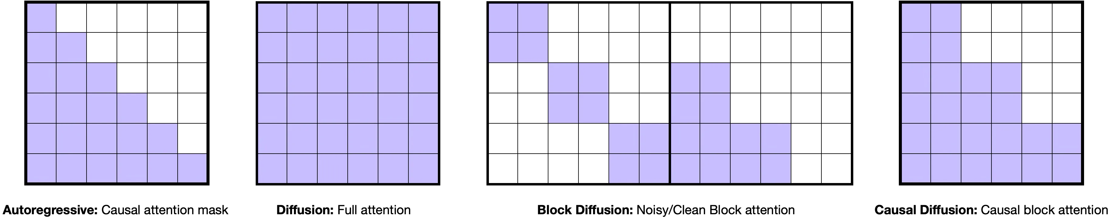
Figure: Attention patterns for Autoregressive, Diffusion, Block Diffusion, and Causal Diffusion language models.
The visual shows how our Causal Diffusion approach (panel 4) creates a block lower triangular attention pattern that combines the best aspects of autoregressive causality with block-level updates.
In practice, Causal Diffusion models are much cheaper to train than Block Diffusion for similar quality. To show this, we trained 246M-parameter Block Diffusion and Causal Diffusion models on the same data and tracked compute and performance over training.

On the left, we plot training tokens vs. estimated FLOPs. Because Block Diffusion carries both a noisy and a clean copy of the sequence, it uses roughly 2× more FLOPs than Causal Diffusion for the same number of tokens.
On the right, we plot training tokens vs. average LM Harness accuracy (HellaSwag, OpenBookQA, ARC-Challenge, PIQA, WinoGrande). For a fixed number of tokens, the two models reach very similar accuracy.
In other words: Causal Diffusion keeps the benefits of Block Diffusion while delivering comparable performance at roughly half the training compute.
Scaling Behavior
So far this has all been about architecture. To decide whether Causal Diffusion is worth scaling, we need to look at performance vs compute.
Setup
We trained three 1.5B-parameter models, one from each family: AR (causal attention), Diffusion LM (full attention), and Causal Diffusion LM (block-causal diffusion). All models were trained on 150B tokens from a subset of Nemotron-CC-HQ subset.
Along the training trajectory we evaluated them on five LM Harness tasks: HellaSwag, OpenBookQA, ARC-Challenge, PIQA, WinoGrande. We use LM Harness rather than validation loss because loss functions differ fundamentally between AR and diffusion models, making direct comparison difficult. For the AR model we use standard log-likelihood scoring. For the diffusion-style models we cannot compute exact likelihoods, so we follow prior work and use Monte Carlo sampling (128 samples) to estimate the likelihood. We report the average LM Harness accuracy across the five tasks.
Accuracy vs Tokens
First, we look at accuracy vs tokens seen:
As training progresses, AR consistently achieves the highest average LM Harness accuracy for a given number of tokens. The standard diffusion model lags behind across most of the trajectory. However, the causal diffusion model sits between the two: noticeably better than the diffusion baseline and closer to AR than to standard diffusion.
More concretely, we find that AR is superior for raw performance per token, but Causal Diffusion is a substantial improvement over full-attention diffusion while retaining the blockwise decoding structure.
Scaling Laws: Error vs Compute
To make the comparison more explicit, we also fit simple scaling laws in compute–error space. We approximate compute as C ≈ 6 N D, where N is the number of non-embedding parameters, D is the number of training tokens seen, and C is the training FLOPs.
For each family, we compute and , where , and fit a straight line , which corresponds to .
The fitted scaling laws are:
- Diffusion LM:
- Causal Diffusion:
- AR:

Two patterns stand out. The Diffusion LM line has a flatter slope (): more compute helps, but more slowly. AR and Causal Diffusion have very similar, but steeper slopes ( and ): both benefit substantially from additional compute. In other words: Causal Diffusion inherits the good scaling behavior of AR models, while diffusion models lag behind.
Where Causal Diffusion Fits
Putting everything together, each approach has distinct trade-offs. Autoregressive LMs achieve the best scaling per FLOP but are inherently one-token-at-a-time. Diffusion LMs support multi-token generation and any-order dependencies but scale worse per unit compute. Block Diffusion LMs fix the train/inference mismatch with block-causal structure but pay roughly 2× compute due to the clean plus noisy halves.
Causal Diffusion LMs keep the block-causal attention and multi-token generation, drop the clean half to become cheaper than Block Diffusion, and show AR-like scaling exponents with respect to compute.
Causal diffusion is a diffusion language model endowed with two properties: autoregressive scaling behavior and multi-token generation. In the next post, this chunkwise view will be crucial for controlling higher-level properties of the output, which are usually expressed over spans rather than single tokens. Our main takeaway is: Causal Diffusion provides the scaling behavior of AR and the blockwise generation of diffusion models.