Tracing the language model’s outputs to training data: In the following demo, PRISM-1.6B decomposes each token it generates into contributions across a handful of prototypes. A prototype is a learned pattern that represents a cluster of similar examples in the training data.

• Each colored slice on the right shows a prototype’s contribution to the logit for the sampled token,
• Together, the slices add up exactly to the final logit,
• Hover over a slice to see the prototype’s broad category (e.g., Medical & Bio), its more specific role (e.g., “physiology”), and its representative training data snippet that most strongly activates it.

Loading prompt analysis…

We show an interactive projection (UMAP) visualization of all 16,384 prototypes that PRISM-1.6B learned. Overall, we observe a prototype dictionary where a bit more than half of the units specialize on low-level morphology and grammatical scaffolding (~35% and ~20%, respectively), while a large minority capture domain-heavy patterns such as medical and biological language (~7%), science and technology (~5%), institutional and civic text (~6%), social and demographic or family descriptions (~3%), named entities (~5%), environment and climate content (~2%), and finance and economics (~1%). Other remaining prototypes concentrate on structured artifacts like numbers and time expressions (~6%), boilerplate fragments (~3%), URLs and identifiers (~2%), and remaining miscellaneous patterns (~3%).

Loading visualization...

We now pick a few prototypes and show the training data snippets they map to.

In the interactive below, each card shows a single learned prototype. The header gives its automatically inferred category and name. For each prototype, we present the top tokens that are most strongly associated with the prototype, and the training data snippets it maps to. We can directly trace any generated token to prototypes, and from there to the training data.

Medical / Biology Science / Tech Numbers / Time Social / Demographic / Family Finance / Econ UX / Meta URLs / IDs Environment / Climate Institutions / Civic / Academic Named Entities

Loading prototypes…

Intervening on prototypes during text generation

In this demo, we pick one prototype and, at every token, clamp its activation so that its contribution to the sampled token’s logit is forced to be a fixed fraction of PRISM’s original top-1 logit. This lets us see directly how amplifying or muting a single, training pattern (for example, “clinical trial boilerplate” or “fraction arithmetic”) changes the model’s behavior. Hover over the text to visualize how the sampled token’s probability shifts as a result of boosting the prototype.

No intervention entries found.

Group prototype intervention, during generation, for science & tech (sky blue) prototypes.

In the demo below, we instead act on an entire labeled category: at each token we inspect the top-16 active prototypes, aggregate the logit signatures of those tagged Science & Tech, and add or subtract a fixed fraction of that aggregate, to amplify or reduce the influence of science and tech patterns wherever they appear in the mixture. Suppressing this category removes the sky blue highlights and shifts the text toward other patterns (such as institutional or civic language), while boosting it produces more science and tech content, like references to web browsers and email infrastructure.

No intervention data found.

Introduction

Generative AI has a data provenance challenge. AI labs have paid record-breaking settlements over training data. Others face ongoing litigation from publishers. When statutory damages reach exorbitant amounts, the question at the center of these cases becomes urgent: when a model generates an output, what training data is it relying on?

This problem, training data attribution (TDA), matters beyond the courtroom. Reliable attribution lets us value data appropriately, understand how LLMs solve hard problems, and verify their outputs. We would prefer a model answering a medical question to rely on journal articles rather than personal blog posts.

Existing approaches based on influence functions and training data attribution that addresses this question. However, these methods often require careful approximations to scale to billion parameter models, and yet struggle to provide reliable insights.

PRISM takes a different approach: it ties training data attribution directly to the model architecture. Every prediction decomposes into a sparse combination of learned prototypes; patterns corresponding to clusters of training examples. The architecture is explicitly constrained so that every output logit can be faithfully traced back to these clusters. Consequently, attributing the model’s output back to the training data is a single forward pass. A medical answer might draw 60% from a prototype grounded in peer-reviewed abstracts; a code completion might trace back to documentation rather than Stack Overflow.

In the sections that follow, we cover PRISM’s architecture and training losses, our automated pipeline for labeling prototypes and retrieving training neighbors, and scaling results from 124M to 1.6B parameters; where PRISM stays within 5% of baseline with under 2% overhead.

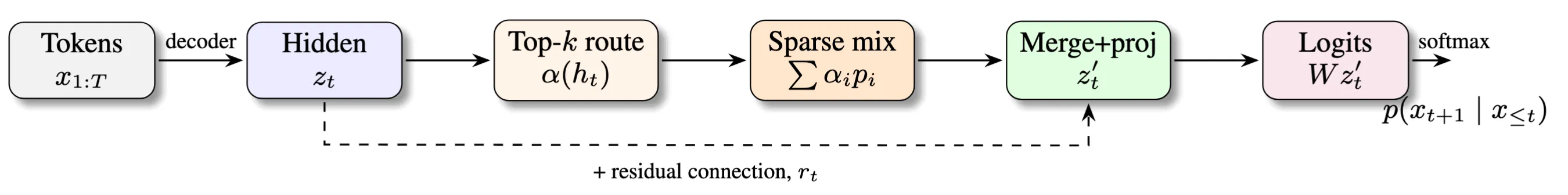
PRISM Architecture & Loss Functions

We now discuss the key technical underpinnings of our approach, introducing the prototype matrix, routing rule, residual path, and training losses.

Standard LM heads collapse all learned patterns into a single dense weight matrix; no row or column corresponds to a reusable training pattern. PRISM asks: what if we made the logit layer an interpretable map of the training data?

We leave the transformer backbone unchanged and only modify the output layer. Instead of sending the final hidden state $z_t$ directly through a dense matrix $W$, we first express $z_t$ as a sparse, non-negative mixture of prototypes plus a residual, then map to logits.

Two components replace the dense LM head:

1. a bank of prototypes, each intended to automatically learn a recurring pattern in the training data while being strongly tied to specific training instances; and
2. a sparse mixing mechanism that, given the current hidden state $z_t$, selects a small set of relevant prototypes and combines their contributions to produce the next-token logits, plus a residual term for whatever is not captured by the prototypes.

Informally: the model asks which few prototypes does this context resemble, and how do they score possible next tokens?

Architecture

To trace the prediction of an LLM back to recurring patterns in the training dataset, we draw inspiration from Prototype Networks,  ^{[1, 2, 3, 4, 5]} [1] Snell et al., 2017. Prototypical Networks for Few-shot Learning [2] Li et al., 2017. Deep Learning for Case-Based Reasoning through Prototypes [3] Chen et al., 2018. This Looks Like That: Deep Learning for Interpretable Image Recognition [4] Ming et al., 2019. ProSeNet: Interpretable and Steerable Sequence Learning via Prototypes [5] Willard et al., 2024. This Looks Better than That: Better Interpretable Models with ProtoPNeXt a family of interpretable models with a long history in deep image classification, that make predictions by comparing the current input to some aspect of the training dataset that was previously seen, yielding explanations in the form this-looks-like-that. Recent work has proposed bringing these ideas to NLP, but progress remains limited to narrow text classification tasks  ^{[6, 7, 8, 9]} [6] Arik & Pfister, 2020. ProtoAttend: Attention-Based Prototypical Learning [7] Das et al., 2022. ProtoTEx: Explaining Model Decisions with Prototype Tensors [8] Hong et al., 2023. ProtoryNet: Interpretable Text Classification via Prototype Trajectories [9] Xie et al., 2023. Proto-lm: A Prototypical Network-Based Framework for Built-in Interpretability in Large Language Models . Large vocabularies and free-form text generation have proven a major barrier in this respect.

The most direct way to bring this-looks-like-that into next-token prediction is to treat it as a $V$-way classification problem: compute $K$ prototype activations and mix them into $V$ vocabulary scores with a dense matrix $M\in\R^{V\times K}$, as in ProtoPNet-style classifiers. This adds $KV$ parameters and $O(KV)$ FLOPs per token on top of the $O(Kd)$ prototype similarity cost; with vocabularies $V\approx 50{,}000$, even moderate $K$ already implies tens to hundreds of millions of new weights (e.g., $K=2{,}000\Rightarrow KV=100\,\text{M}$), making this approach prohibitively expensive at language-model scale.

PRISM’s head instead keeps computation in the model’s embedding space, forming a reconstruction

$$\hat{z}_t=\sum_k \alpha_{t,k} p_k$$

and applying $W\in\R^{ V\times d}$ to obtain logits: $W\hat{z}_t=(WP)\alpha_t$. This is functionally equivalent to a ProtoPNet style mixer with $M=WP$ while yielding significant parameter reduction (e.g., $d\approx 500\Rightarrow Kd+d V=1\text{M}+25\text{M}$, or $1\text{M}$ with weight-tying), and preserving metric continuity by avoiding a coarse $d\!\to\!K\!\to\! V$ switch. Empirically, we find that this reparameterization trains faster and more smoothly. On toy experiments with the TinyStories dataset, the ProtoPNet style head required up to $3\times$ longer wallclock time to reach the same perplexity.

Following the literature, we adopt an autoregressive backbone as input to the prototype layer. Our modifications are restricted to the final layer, so PRISM can be implemented in a way that is compatible with standard transformer training recipes and, in principle, could also be adapted to other sequence models such as diffusion based language models. We train the entire model end-to-end, allowing PRISM to learn its own prototypical representation of inputs.

Positive similarity scoring and top-$k$ routing

Once the backbone GPT model has processed the current input, the prototype layer computes the similarity of the input $\,z_t\,$ to every prototype in the bank $[p_1,\dots,p_K]$. For each prototype, compute its cosine similarity to the current state, $z_t$

$$c_{t,i}\;=\;\frac{z_t^\top p_i}{\|z_t\|_2\,\|p_i\|_2}\quad\text{for }i\in[K]$$

We apply an optional learned scalar $\tau\!\in\!\R_{>0}$ to expand the effective dynamic range of cosine scores. Intuitively, we want the model to expose non-negative reasoning : predictions are explained as this-looks-like-that  (positive evidence from similar prototypes) rather than this-does-not-look-like-that  (subtractive evidence). Thus, we enforce non-negativity via a rectifier:

$$\tilde\alpha_{t,i}\;=\;\mathrm{ReLU}(\tau\,c_{t,i})$$

We select the index set $\mathcal{K}_t=\operatorname{TopK}(\{\tilde\alpha_{t,i}\}_{i=1}^K,k)$ and define the final, few-hot similarities

$$\alpha_{t,i}\;=\;\tilde\alpha_{t,i}\,\mathbf{1}\{i\in\mathcal{K}_t\}$$

This top-$k$ routing ensures that each token prediction is explained in terms of a small, human-readable set of prototypes rather than a dense mixture over all $K$.

Sparse reconstruction

We would like to reason about a prediction using as few prototypical contexts as possible, to enable crisp interpretability. Sparse activations encourage each prototype to specialize and represent tighter clusters of the training data, which makes it easier to summarize what the model is “thinking” in terms of a handful of distinct patterns i.e. the prototype logit signatures become more fine-grained. Given the $k$ most similar prototypes, we form a $k$-sparse reconstruction

$$\hat{z}_t\;=\;P\,\alpha_t\;=\;\sum_{i\in\mathcal{K}_t}\alpha_{t,i}\,p_i\;\in\;\R^d$$

This follows existing SAE literature, which learns sparse dictionaries for hidden states at intermediate layers. In contrast, PRISM learns a sparse dictionary of training-grounded prototypes that directly explain the model’s output logits without a separate decoder. The features learned are also directly tied to groups of training examples (see next section).

Merge and logits

We use a residual merge with the original state to account for parts of the input not reconstructed by prototypes. The residual $r_t=z_t-\hat{z}_t$ is computed as the difference between the original $z_t$ and the reconstruction $\hat{z}_t$ (thus, $z'_t=z_t$). The vocabulary projection is standard:

$$z'_t \;=\; \hat{z}_t+r_t\qquad\rightarrow\qquad \ell_t \;=\; W\,z'_t \qquad\rightarrow\qquad p(x_{t+1}\!\mid x_{\le t})=\mathrm{softmax}(\ell_t).$$

Keeping an explicit residual path preserves the expressivity of the original backbone. Rare or input-dependent tokens need not be forced through the prototype dictionary. Measuring how much of each prediction is accounted for by prototypes versus the residual is straightforward.

Faithful Logit decomposition

The PRISM head builds an interpretable logit map at the model’s final layer, ensuring that we can directly quantify the effect and importance of any prototype to any output token by design. By linearity of $W$, the next-token logits decompose into per-prototype contributions:

$$\ell_t = Wr_t + \sum_{i\in\mathcal{K}_t}\alpha_{t,i}(Wp_i)$$

Each prototype $p_i$ thus induces a fixed token–logit signature $W p_i\in\R^V$, and the model’s prediction is an explicit, sparse, non-negative mixture over at most $k$ such signatures. This yields additive, causally faithful units that can be ablated or amplified directly at the logit level. When a model predicts a given token, we can recover a given prototype’s exact contribution simply by multiplying its input activation $\alpha_{t,i}$ by its fixed logit signature $Wp_i$ (indexed at the predicted token). As a matter of preference, we combine the scalar $\tau$ into $Wp_i$ when interpreting the prototype signature. This restricts our interpretation of the final logits to a weighted superposition in the range $[0,1]$ of top-$k$ prototype signatures.

Loss functions

Here we detail the loss functions used to train PRISM. Let $\mathcal{I}(\mathcal{B})$ denote the index set of token positions across the current macro-batch. Additionally, let $d_i(j)=-c(p_i, z_j)$ be the negative cosine distance between prototype $i$ and the token representation at position $j\in\mathcal{I}(\mathcal{B})$.

$$\mathcal{L}_\text{PRISM} = \mathcal{L}_\text{CE} + \underbrace{\mathcal{L}_{R_1} + \mathcal{L}_{R_2}}_{\text{Clustering Losses}} + \mathcal{L}_\text{RES}$$

Cross-Entropy ($\mathcal{L}_{\mathrm{CE}}$).

We use the standard objective

$$-\frac{1}{|\mathcal{B}|}\sum_{(x_{1:T})\in\mathcal{B}} \sum_{t=1}^{T-1}\log p_\theta\!\left(x_{t+1}\mid x_{\le t}\right)$$

where $p_\theta(x_{t+1}\mid x_{\le t})=\mathrm{softmax}(\ell_t)_{x_{t+1}}$ and $\ell_t$ are the logits computed from the merged state $z'_t$.

Prototype Pull ($\mathcal{L}_{R_1}$).

We encourage each prototype to anchor to some token in the batch with

$$\mathcal{L}_{R_1} =\frac{1}{K}\sum_{i=1}^{K}\min_{j\in\mathcal{I}(\mathcal{B})} d_i(j).$$

Training-Point Pull ($\mathcal{L}_{R_2}$).

Symmetrically, every token position should be close to at least one prototype via

$$\mathcal{L}_{R_2} =\frac{1}{|\mathcal{I}(\mathcal{B})|}\sum_{j\in\mathcal{I}(\mathcal{B})} \min_{i\in[K]} d_i(j).$$

Combined, the $R_1$ and $R_2$ terms can be viewed as clustering losses in the backbone LM’s final layer embedding.

Residual ($\mathcal{L}_{\mathrm{RES}}$).

We set $z'_t=\hat{z}_t+r_t$ with $r_t:=z_t-\hat{z}_t$. We simply minimize the mean-squared residual

$$\mathcal{L}_{\mathrm{RES}} \;=\; \|r_t\|_2^2 \;=\; \|z_t-\sum_{i\in\mathcal{K}_t}\alpha_{t,i}\,p_i\|_2^2$$

i.e., the MSE of the mismatch between the prototype reconstruction and the original state.

(Optional) Prototype Diversity ($\mathcal{L}_{\mathrm{DIV}}$).

We optionally encourage prototypes to cover diverse representations within the final layer’s embedding, to reduce prototype overlap and encourage specialization. For this setting, we penalize off-diagonal coherence of the $\ell_2$-normalized prototypes. With $\tilde{p}_i=p_i/\|p_i\|_2$ and $G=\tilde{P}^{\top}\tilde{P}$, $\mathcal{L}_{\mathrm{DIV}}=\frac{1}{K(K-1)}\sum_{i\neq j} G_{ij}^{2}$. For $K>D$, the average squared coherence is lower bounded by the Welch bound  ^[10] [10] Welch, 1974. Lower bounds on the maximum cross correlation of signals . Driving $\mathcal{L}_{\mathrm{DIV}}$ toward this limit spreads prototypes nearly optimally on $\mathbb{S}^{D-1}$ and empirically yields crisper, more distinct roles without harming validation cross-entropy.

Training Data Attribution in a Single Forward Pass

PRISM exposes all quantities needed for attribution during inference. Given hidden state $z_t$:

$$c_{t,i}=\frac{z_t^\top p_i}{\|z_t\|_2\|p_i\|_2},\qquad \tilde\alpha_{t,i}=\mathrm{ReLU}(\tau c_{t,i}),\qquad K_t=\operatorname{TopK}(\{\tilde\alpha_{t,i}\}_{i=1}^K,k)$$

The attribution measure over training data is:

$$\mathcal{A}_t = \sum_{i\in K_t}\alpha_{t,i}\,\mu_{S_i}$$

where $S_i$ is the precomputed set of training tokens nearest to prototype $i$, and $\mu_{S_i}$ is a weighting over that set (commonly uniform). $\mathcal{A}_t$ is fully determined by forward pass values and static mappings. No gradients, no Hessians, no dataset search.

Automated Interpretability Pipeline

PRISM gives us two handles for automation: each prototype is tied to training contexts via its activations, and each has a fixed logit signature $Wp_i$ over the vocabulary. We use these to (i) find training snippets each prototype represents, and (ii) assign human-readable labels.

Nearest Neighbor Search

For each prototype, we recover concrete training examples with a single streaming pass over the dataset. We retain the top-$L$ positions with highest activations:

• For every token position $j$, compute $\alpha_{j,i}$ for all prototypes
• Maintain a max-heap of size $L$ per prototype storing best matches
• Enforce distinct-position constraints to avoid redundant sliding-window variants

This is a one-pass $O(NK)$ procedure with $O(KL)$ memory. Because the $\mathcal{L}_{R1}$ loss pulls each prototype toward training tokens, high-activation neighbors exist by construction. In practice, similarity converges after scanning roughly 1% of training data.

Automatic Labeling

For each prototype, we build a compact “card” containing (i) top tokens from its logit signature and (ii) local contexts where it fires. A small labeling model converts this into human-readable metadata: a short name, a one-line description (e.g., “clinical trial boilerplate”, “Unix timestamps”), and example contexts.

A second pass assigns coarse tags used in visualizations: broad category (Science & Tech, Numbers & Time, URLs & IDs), syntactic role (noun-like, function word, scaffold phrase), and optional domain tags (medical, US universities). This runs offline on learned prototypes and their neighbors.

Performance & Scaling

We now discuss the training procedure and performance details from training PRISM end-to-end across various model sizes.

Scaling from 124M to 1.6B

Overview of PRISM performance compared to an unconstrained GPT model
We train GPT backbones from 124M to 1.6B parameters end-to-end with the prototype layer for one epoch on FineWeb-Edu-10B. PRISM stays within 5% of unconstrained baselines on validation loss and downstream benchmarks across all scales. The prototype layer adds $d \times K$ parameters: at GPT-XL scale with $K=16384$ prototypes, this is 26M parameters (1.7% overhead). Training time increases by less than 2%. The overhead shrinks as a fraction of total parameters as backbones scale up. Faithful attribution to training data does not require sacrificing model quality.

Conclusion

PRISM demonstrates that training data attribution doesn’t have to be a post-hoc approximation bolted onto an opaque model. By building interpretability into the architecture, we get faithful explanations at the cost of a single forward pass. At 1.6B parameters, PRISM stays within 5% of baseline performance with under 2% overhead. The prototype dictionary is inspectable, editable, and directly tied to training data. This works lays a foundation for language models that can be more easily audited, steered, and whose predictions can be faithfully traced to the training data.

Our results indicate that, at GPT XL scale, there are solutions comfortably within 5% of the original backbone’s performance that satisfy PRISM’s interpretability constraints. In this view, PRISM does not enforce an accuracy–interpretability tradeoff so much as bias optimization toward a part of the Rashomon set where the logit layer admits a structured, training-data–grounded decomposition into prototypes.