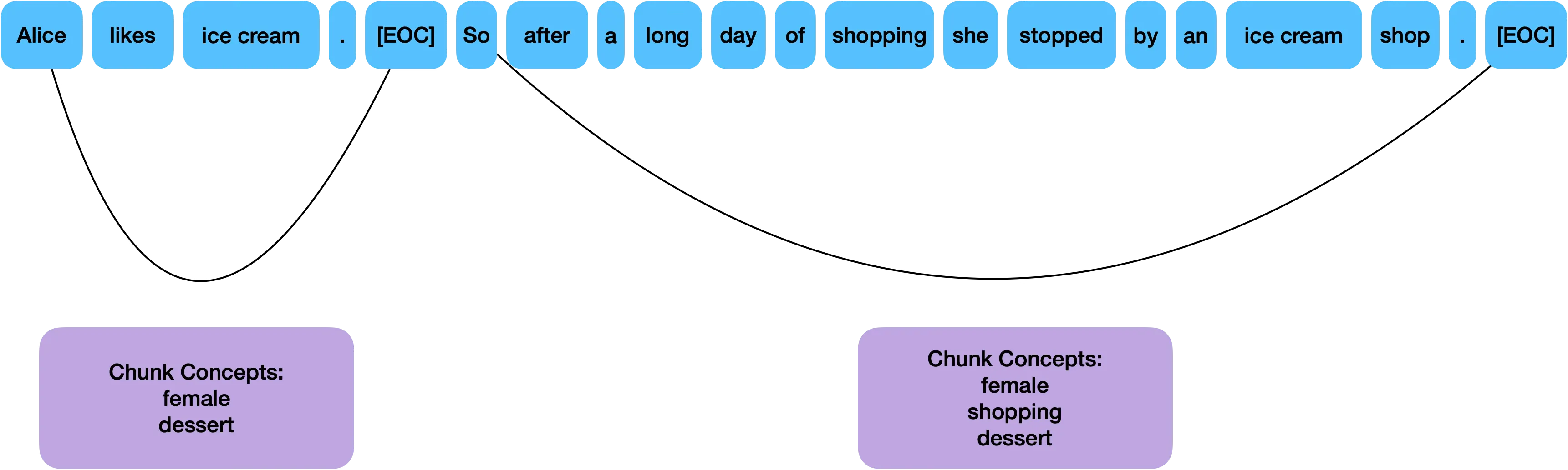
Below, we show example generations from a base model (not instruction fine-tuned), along with human understandable concept explanations for groups of tokens (chunks) that are generated by the model.

Loading attribution data...

Overall, our model natively decomposes the model’s representations into human-understandable concepts. Below we show a selection of concepts that our model learned and the most important tokens associated with those concepts. Even though we constrain the model to learn human-understandable concepts, it is still able to discover new concepts; we highlight a few of them here.

All (0) ● Known ◆ Discovered

‹

›

Importantly, we demonstrate that our model enables unlearning potentially undesirable concepts through concept interventions. Below, we show a few examples where intervention led to a removal of an unwanted concept.

Introduction

Language models are inscrutable black boxes. Billions of parameters transform input tokens into output probabilities, with little visibility into why a particular answer was produced, which parts of the prompt mattered, or how to reliably steer the model toward or away from specific behaviors.

The standard response is post-hoc interpretability: train your model, then try to reverse-engineer what it learned. This approach offers partial, often unreliable glimpses into behavior. At Guide Labs, we take a different path: interpretability has to be designed in; from architecture to training objective to the structure of the data itself.

This post describes the concept module, an architectural bottleneck that forces every prediction through human-interpretable concepts. We’ve scaled this design to 8 billion parameters and found that interpretability behaves like a fixed tax: a small, constant overhead that preserves scaling laws. You don’t have to choose between capability and transparency.

The concept module gives us three things current models lack:

• Faithful explanations: The linear path from concepts to logits lets us compute exact, additive contributions of each concept to any output; not approximations, not post-hoc rationalizations.
• Debugging and failure analysis: When the model misbehaves, we can see which concepts fired and why. We can distinguish bad concepts from spurious input features.
• Steerable generation: We can adjust concept activations at inference time to directly control outputs; suppress toxicity, boost technical detail, or perform surgical edits without retraining.

Below, we describe the architecture and training objectives that make this possible, then show empirically that the approach scales

The Concept Module

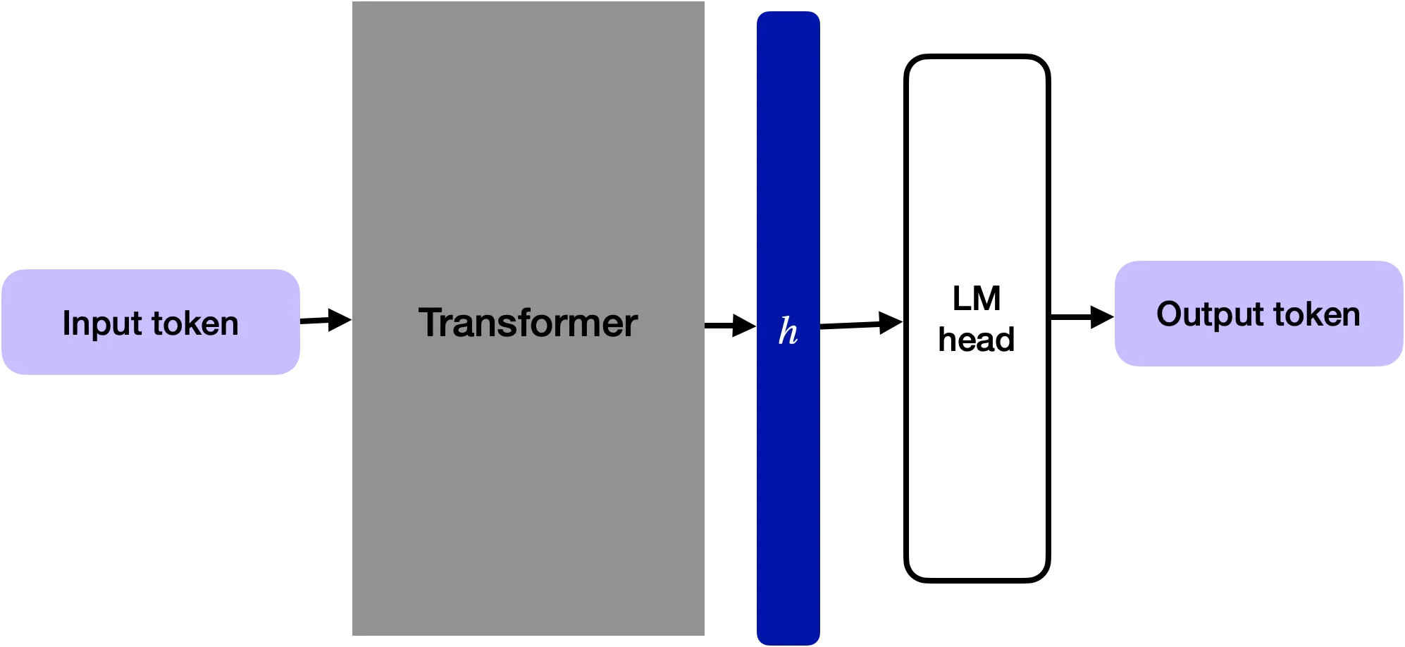
The concept module is a thin bottleneck that sits between the transformer backbone and the output head. The transformer still maps tokens to hidden states as usual, but instead of sending those hidden states straight to the LM head, we:

1. express them in terms of concept activations,
2. reconstruct a new hidden state as a linear combination of concept embeddings, and
3. only then feed this reconstructed state into the LM head.

Given a language model setting, AR or Diffusion, we cut the direct path from hidden state to logits. Insert a narrow “concept layer” in the middle. Train the model end-to-end from scratch. Once this is done, every prediction must go through concepts and we can both inspect and edit those concepts.

Data Setup

We assume a pretraining corpus that is divided into chunks, separated by a special end-of-chunk token [EOC]. For each chunk we have a set of known concept labels (for example: legal, medical, politeness, apology). The labels are chunk-level and positive-only: annotated positives are trusted as “present”; everything else is “unknown” rather than “negative”. We described the system, ATLAS, that we built to accomplish this in a previous post.

During training the model assigns token-level probabilities to concepts, but these are only constrained via the chunk-level labels; we never require token-level annotations.

Architecture

We start from any transformer language model.

Let $h \in \mathbb{R}^d$ be the hidden state for a token (after the backbone). In a vanilla LM, $h$ goes straight into the LM head to predict the next token. With the concept module, that direct path is removed. Instead, $h$ is routed through a concept bottleneck.

From Hidden States to Concepts

We add two small heads:

• $f(h)$ for known concepts,
• $g(h)$ for unknown concepts.

Their sigmoid outputs give activation probabilities

$k = \sigma(f(h)) \in \mathbb{R}^n, \qquad u = \sigma(g(h)) \in \mathbb{R}^m,$

where $n$ is the number of known (labelled) concepts and $m$ is the number of unknown concepts, typically $m \gg n$. Each dimension is an independent Bernoulli variable: present or absent.

Concept activations to embeddings

Each concept has a learned embedding, analogous to token embeddings:

• $K \in \mathbb{R}^{d \times n}$ with columns $K_i$ for known concepts,
• $U \in \mathbb{R}^{d \times m}$ with columns $U_j$ for unknown concepts.

We form concept-weighted embeddings:

$$\hat{k} = \sum_{i=1}^{n} k_i K_i, \qquad \hat{u} = \sum_{j=1}^{m} u_j U_j.$$

Reconstructing the hidden state

We reconstruct a concept-based hidden state

$\bar{h} = \hat{k} + \hat{u}$

and feed $\bar{h}$ (not $h$) into the LM head to predict the token.

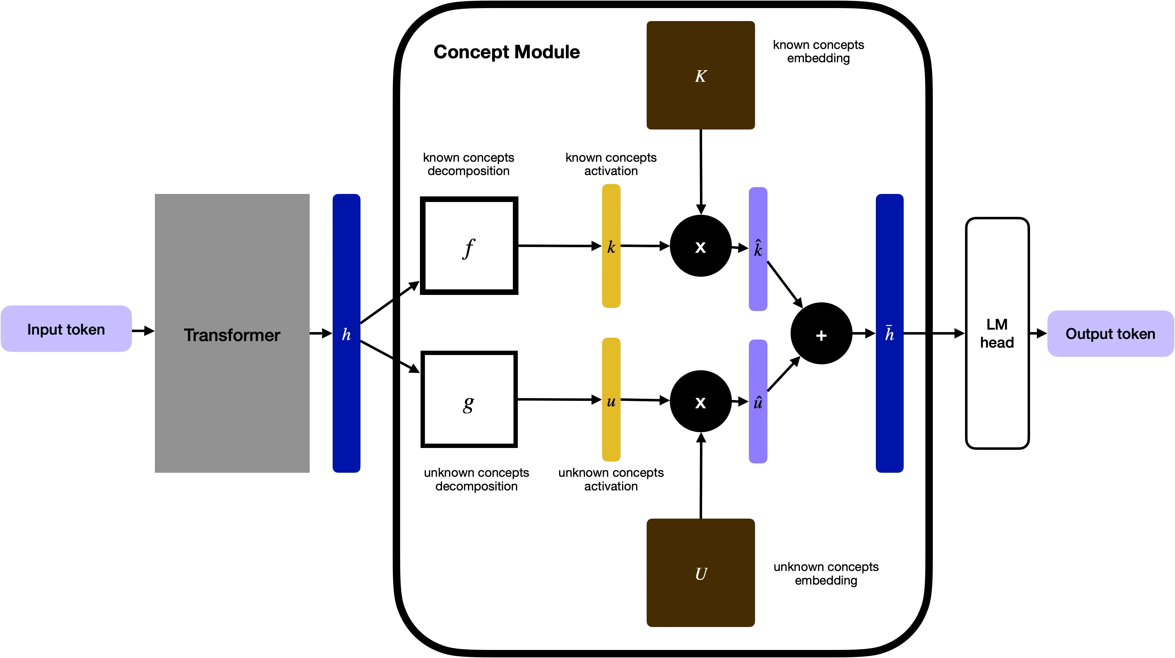
Enables simutaneous concept-based explanation and control: our proposed architectural design has an important consequence; every logit is now a linear function of concept activations and concept embeddings, which directly translates to exact and attribution and direct control.

Training Objectives

With the model’s architecture set, we now switch to discussing the associated training objectives that constrain the models towards satisfying the proposed interpretability requirements. We train the backbone and concept module jointly with four losses.

1. Language modelling loss

$\mathcal{L}_{\text{token}}$ is the masked token prediction (or next-token for AR) objective, but applied to $\bar{h}$. This keeps overall language modelling quality high.

2. Concept presence loss

Our labels say which concepts appear somewhere in a chunk, not where. For concept $c$, let $p_{c,t}$ be its predicted probability at token $t$ in the chunk. The probability that $c$ appears at least once is

$P_c^{\text{chunk}} = 1 - \prod_{t \in \text{chunk}} (1 - p_{c,t}).$

We compare $P_c^{\text{chunk}}$ to the binary chunk-level label with a standard binary cross-entropy loss, summed over known concepts. This encourages the token-level scores to “light up” within the chunk in a way that makes the aggregated probability match the labels.

3. Independence loss

We would like known and unknown concepts to encode different aspects of $h$. For a minibatch of size $B$, let $\hat{k}, \hat{u} \in \mathbb{R}^{B \times d}$ be the batch matrices of known and unknown embeddings, and $\mu_{\hat{k}}, \mu_{\hat{u}}$ their column means. We penalise their cross-covariance:

$$\mathcal{L}_{\text{indep}} = \left\lVert \frac{1}{B-1} (\hat{k} - \mathbf{1}\mu{\hat{k}}^\top)^\top (\hat{u} - \mathbf{1}\mu_{\hat{u}}^\top) \right\rVert_F^2.$$

Intuitively, if a pattern is already explained by known concepts, this discourages the model from redundantly encoding it in the unknown space.

4. Residual reconstruction loss

Given ground-truth known concept labels $k^{\text{gt}}$, the “ideal” known embedding for a hidden state is

$\hat{k}_{\text{gt}} = \sum_{i=1}^{n} k_i^{\text{gt}} K_i.$

We interpret the unknown embedding as the residual $\hat{u}^{\text{gt}} = h - \hat{k}^{\text{gt}}.$

We train the unknown head so that its prediction $\hat{u}$ matches this residual:

$$\mathcal{L}_{\text{rec}} = \lVert \hat{u} - \hat{u}^{\text{gt}} \rVert_2^2.$$

Complete Loss. Putting everything together, the full loss is:

$$\mathcal{L}= \mathcal{L}_{\text{token}} + \lambda_{\text{concept}} \mathcal{L}_{\text{concept}}+ \lambda_{\text{indep}}\mathcal{L}_{\text{indep}}+ \lambda_{\text{rec}} \mathcal{L}_{\text{rec}}.$$

After training with this objective, the base LM becomes concept-based by construction: every prediction is mediated by concept activations and embeddings.

Attribution and Steering

With the concept module in place, we get a clean, algebraic handle on how the model uses concepts and inputs to produce outputs.

Concept Attribution

As we previously mentioned, the model has a linear path from concepts to output logits: $\bar{h}$ is a linear combination of concept embeddings so each output logit decomposes into a sum of per-concept terms. Let $w_i$ be the activation of concept $c_i$, $v_i$ its embedding, and $w_{y_j}$ the LM-head weight vector for output token $y_j$. Then the contribution of concept $c_i$ to the logit of $y_j$ is

$$C(c_i, y_j) = w_i \cdot (v_i^\top w_{y_j}).$$

Summing over $i$ recovers the total logit for $y_j$.

Feature attribution (prompt tokens → output tokens)

Inspired by [1], we implement Integrated Gradients [2] to compute feature attribution. For this we use Integrated Gradients on token embeddings. For an input token $x_t$ with embedding $T_{x_t}$, baseline embedding $T_{[\text{MASK}]}$, and output token $y_j$:

• Define interpolation points $T^{(p)} = T_{[\text{MASK}]} + \frac{p}{P}(T_{x_t} - T_{[\text{MASK}]}) \in ℝ^{d}$ for $p = 1, \dots, P$.
• The attribution of $x_t$ to $y_j$ is

$C(x_t, y_j) = \frac{1}{P} \sum_{p=1}^{P} (T_{x_t} - T_{[\text{MASK}]})^\top \nabla_{T^{(p)}} \text{logit}_{y_j}.$

Given that our model is trained with [MASK], the [MASK] serves as a natural baseline: it represents “no meaningful information”, and we measure how much moving to the actual token shifts the logit.

Input-to-Concept Attribution

We also implement Integrated Gradients [2] to compute the input-to-concept attribution. We reuse Integrated Gradients, but with the concept activation $w_i$ as the scalar output:

$$C(x_t, c_i) = \frac{1}{P} \sum_{p=1}^{P} (T_{x_t} - T_{[\text{MASK}]})^\top \nabla_{T^{(p)}} w_i.$$

Together with concept attribution, this lets us trace a full chain:

input tokens → concept activations → output tokens.

Concept-level Steering

The same linear structure that makes attribution easy also makes control easy. For an output token $y_j$ we can write:

$\text{logit}(y_j) = \sum_{i} w_i \cdot (v_i^\top w_{y_j}).$

At inference time we are free to modify the activations $w_i$ before they feed into this sum. We can clamp selected concepts to zero (suppressing their influence), rescale helpful concepts up or down, or apply more structured interventions. This is very different from prompt engineering or RLHF: we are not nudging the model and hoping it responds; we are directly editing the internal variables that determine the output.

Performance Scaling Behavior

Interpretability, in this design, behaves like a fixed tax, not a fundamental limitation. You pay a small, predictable premium for being able to see and steer the model’s concepts but you still get essentially the same returns from making the model bigger and training it longer. We demonstrate this through experiments across two model families:

• an autoregressive (AR) family with causal attention, and
• a causal diffusion (CDLM) family with block-causal attention.

For each family we trained three sizes (Small, Medium, Large) and, for each size, a base model and a concept-module model with the same transformer backbone.

Parameter overhead

The concept module keeps the transformer core (depth, width, heads, etc.) unchanged and adds two shallow projection heads plus a bank of concept embeddings. At small scales this module is a noticeable fraction of total parameters. As the backbone grows, its relative share shrinks quickly: the overhead grows much more slowly than the rest of the model.

The more important question is whether this overhead hurts scaling.

Performance comparison

All models were trained on the same data and evaluated throughout training on five LM Harness tasks: HellaSwag, OpenBookQA, ARC-Challenge, PIQA, and WinoGrande. We report average LM Harness accuracy across these tasks.

Autoregressive language model family

Diffusion language model family

Across all sizes in both families, the base and concept-module curves almost overlap. Their learning curves have nearly the same shape, and the gap in average accuracy is small at all points, especially for larger models. Empirically we show that you can add the concept module without breaking the model’s ability to improve with more data.

Scaling law analysis

To quantify this, we fit simple scaling laws relating compute and performance.

We approximate training compute as

$C \approx 6 N D,$

where $N$ is the non-embedding parameter count, $D$ is the number of training tokens, and $C$ is measured in FLOPs up to a constant.

For each family and variant we fit power laws

$\log_{10}(\text{metric}) = a + b \log_{10}(C) \quad\Longleftrightarrow\quad \text{metric} \approx 10^a C^b$

for two metrics: validation loss, and LM Harness error (1 minus the average accuracy over the five tasks).

For the AR family, validation loss follows

• base AR: $\text{loss} \approx 10^{1.329} C^{-0.043}$,
• AR + concept module: $\text{loss} \approx 10^{1.372} C^{-0.045}$;

while LM Harness error follows

• base AR: $\text{error} \approx 10^{0.916} C^{-0.060}$,
• AR + concept module: $\text{error} \approx 10^{1.038} C^{-0.066}$.

For the Diffusion language model family, validation loss follows

• base CDLM: $\text{loss} \approx 10^{1.727} C^{-0.061}$,
• CDLM + concept module: $\text{loss} \approx 10^{1.747} C^{-0.061}$;

and LM Harness error follows

• base CDLM: $\text{error} \approx 10^{0.650} C^{-0.045}$,
• CDLM + concept module: $\text{error} \approx 10^{0.626} C^{-0.043}$.

In both families, the base and concept-module lines are essentially parallel in log–log space. The scaling exponents $b$ stay in the same range, which means both variants benefit from additional compute at similar rates. The concept module mostly shows up as a small vertical shift: a modest constant penalty in loss or error at fixed FLOPs.

Interpretability Scaling Laws

One might expect interpretability to degrade as models grow. Larger networks have more capacity to route around bottlenecks and blur whatever structure you’ve imposed. To test whether this happens, we track two properties: whether concepts remain meaningful (interpretability) and whether pathways stay cleanly separated (disentanglement).

Interpretability: Concept Detection
Concept detection stays flat across model sizes. We measure how reliably the concept module detects concepts by computing segment-level AUC against ground-truth annotations, where higher values indicate more accurate detection.

Interpretability: Token Control
Token control tells a similar story. Here we measure how focused each concept’s influence is on specific vocabulary items: the relative probability mass a concept places on its top-10 tokens through the LM head. Higher values mean sharper, more selective control. Concepts don’t become diffuse as models grow.

Disentanglement: Independence Loss (HSIC)
Turning to disentanglement, we use the Hilbert-Schmidt Independence Criterion to quantify how much the concept module representations correlate with the residual. Lower HSIC values indicate better independence between pathways. Counter-intuitively, this independence actually improves with scale.

Disentanglement: Probing Gap
Finally, the probing gap measures the interpretability benefit of the concept module directly: the AUC difference when probing concept representations versus residual representations for the same detection task. A positive gap means the concept pathway carries signal the residual doesn’t. That advantage holds at scale.

Conclusion

Taken together, these results demonstrate that adding a concept module can make foundation models interpretable without sacrificing scale. We will release Steerling-8B, early 2026, an 8B-parameter causal diffusion model trained from scratch with the concept module.