Interpretability Has Scaling Laws

We show that model interpretability follows a simple, fine-grained, empirical scaling law. First, we tease apart the effect of the two main components of a training compute budget, model size (parameters) and amount of data (tokens), on several key interpretability properties of a model. The larger the interpretable model, the more cleanly it separates human-understandable concepts, and the more reliably it learns them in the first place. This result runs counter to the prevailing expectation that larger models are harder to interpret. On the other hand: data buys human alignment. The more data an interpretable model is trained on, the closer its representations come to mean what a human label would say. These counterintuitive results are a direct consequence of a new way to train models that imposes these constraints during training. We refer readers to our technical report.
Below is an interactive surface over parameters and tokens for each of the four properties, with gold indicating better values. The dashed diagonal is a fixed compute budget. Moving along it trades parameters for tokens, and the four properties do not agree on which direction to move.
Does the concept module detect the right concepts?
We trained interpretable language model families across three orders of magnitude of compute and fit scaling laws to four interpretability properties, separating the effect of model size (parameters) from training data. We find:
- Larger models are able to learn more disentangled representations. Our underlying architecture and training objective enables larger models to more cleanly disentangle concepts in its representation.
- Larger models learn more human-understandable concepts more reliably. At a fixed compute budget, increase in parameters directly improves concept learnability. A bigger model assigns the right human-labeled concepts to text it has not seen before.
- More training data improves human alignment. The more data the model sees, the more closely its learned concept embeddings correspond to the meanings assigned by humans.
- Both data and model size affect how much the model’s output depends on human-understandable concepts. With increasing compute, the model routes a larger share of its prediction through its interpretable embeddings.
What scaling laws currently tell you
Empirical scaling laws that forecast a model’s downstream performance have become a key tool in how model-training teams plan a training run. Given a training recipe that includes the typical primitives: an architecture, optimizer, data mixture, and performance measure, these laws help to forecast how much model size, training data, and compute are needed to reach a target level of performance.
Existing scaling laws typically forecast validation loss or downstream capability. However, if we are interested in whether a model gets more aligned, easier to steer, and learns more disentangled representations with scale, current scaling laws are unhelpful.
A long-standing observation is that neural networks encode concepts in a distributed manner, and in modern transformers this has come to be characterized as superposition, i.e more learned directions than dimensions packed into overlapping subspaces. It is unclear which structure or objective in the standard training pipeline determines this property, since nothing in the pipeline asks for it. Consequently, the standard practice has been to reverse engineer these models, and expect the problem to worsen with scale as a larger model packs more features into the same space. In this post, we discuss a new training recipe that reverses this trend entirely.
A training recipe that makes interpretability measurable
At Guide Labs, we have introduced a training recipe that makes interpretability a constraint of the training process rather than an analysis performed after training. We have described the full recipe in our technical report and previous posts. Here, three parts matter.
First, we annotate the pretraining data with a fixed library of more than 33,000 human-understandable concepts. This gives the model a common concept vocabulary that remains stable across model sizes and training runs.
Second, we place an explicit concept module between the transformer backbone and the language-modeling head.

Steerling’s embedding decomposition: the model representation is split into three interpretable components: known concepts, discovered concepts, and the residual — which together account for every prediction.
The module reconstructs the transformer representation as the sum of three parts:
where contains concepts from the human-labeled library, contains additional concepts discovered by the model, and is the remaining residual.
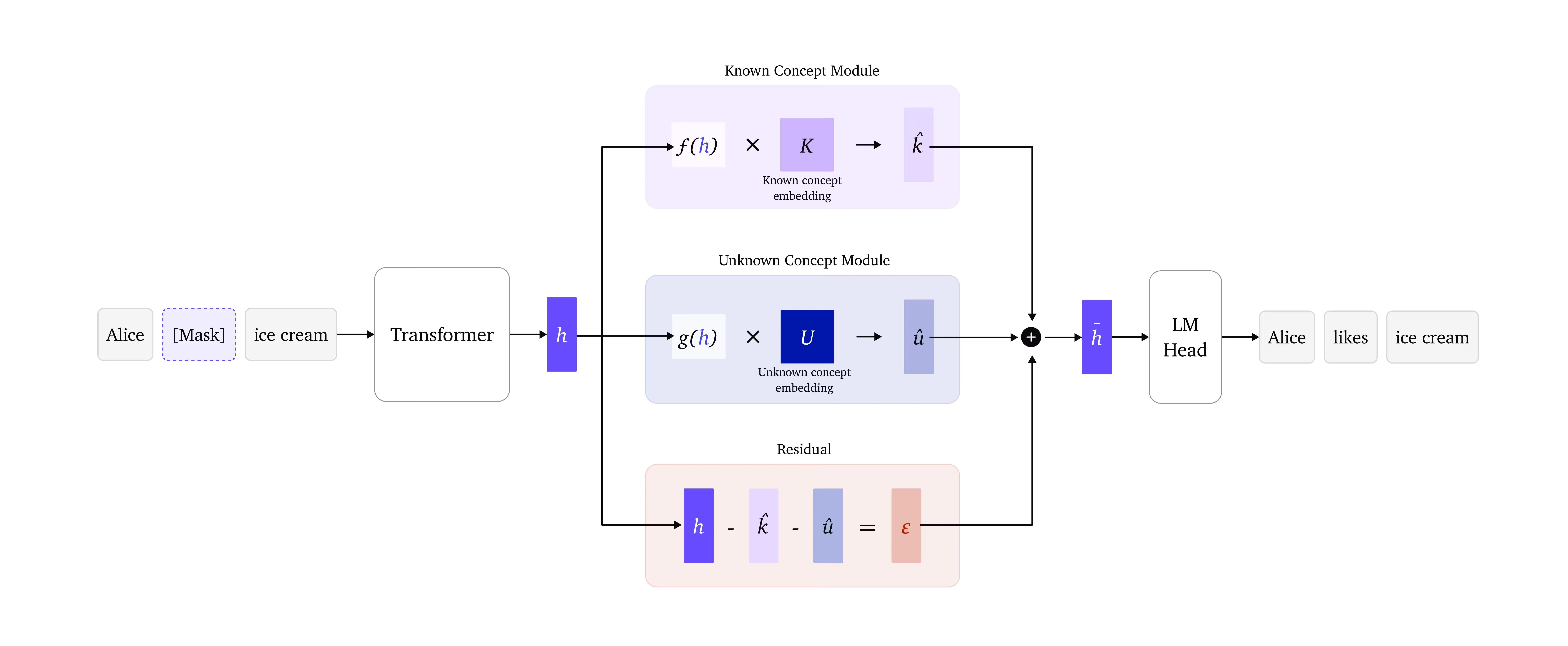
The concept module: showing the known, unknown, and the residual components for a causal diffusion language model.
Third, we train the backbone and concept module together. Alongside the language-modeling objective, the recipe trains the model to detect known concepts, reconstruct the hidden state, and keep the known and discovered representations from encoding redundant information.
Because the output head is linear, the contribution of these three parts to any output logit decomposes exactly:
Given this recipe: we can therefore compare their properties across model sizes, token budgets, compute budgets, and model families.
Four key properties of this new paradigm
We evaluate four properties. Together, they test whether the concept module recognizes the right concepts, keeps its representations separate, accounts for the prediction, and attaches human meaning to the concepts it learns.
-
Concept Detection: this metric corresponds to the Concept loss. It measures whether the model assigns the correct human-labeled concepts to text it has not seen before. Lower is better.
-
Concept Separation: this metric corresponds to the Concept Independence Loss. It measures whether the concept module keeps the known and discovered concept pathways complementary rather than redundant. Lower is better.
-
Concept Contribution: this metric measures how much of the output prediction depends on the known and discovered concepts rather than through the residual. Higher is better.
-
Concept–Language Alignment: this metric corresponds to Known Concept Alignment. It measures whether words and tokens most strongly promoted for a given learned concept embedding match the concept’s human-assigned label and description? Higher is better.
These metrics test four necessary properties of the specific interface that the architecture was trained to provide.
A coarse scaling law
Before separating the effects of parameters and data, we first ask a simpler question: do these properties improve with total training compute?
We fit each metric to a compute-only scaling law:
where is training compute, is the value the metric approaches with scale, and determines how quickly it approaches that value.
Across both autoregressive and causal-diffusion models, all four properties move in the favorable direction as compute increases. The concept module detects concepts more accurately. The known and discovered representations become more distinct. More of the prediction passes through the concept module. The learned concept embeddings become more closely aligned with human-assigned meanings.
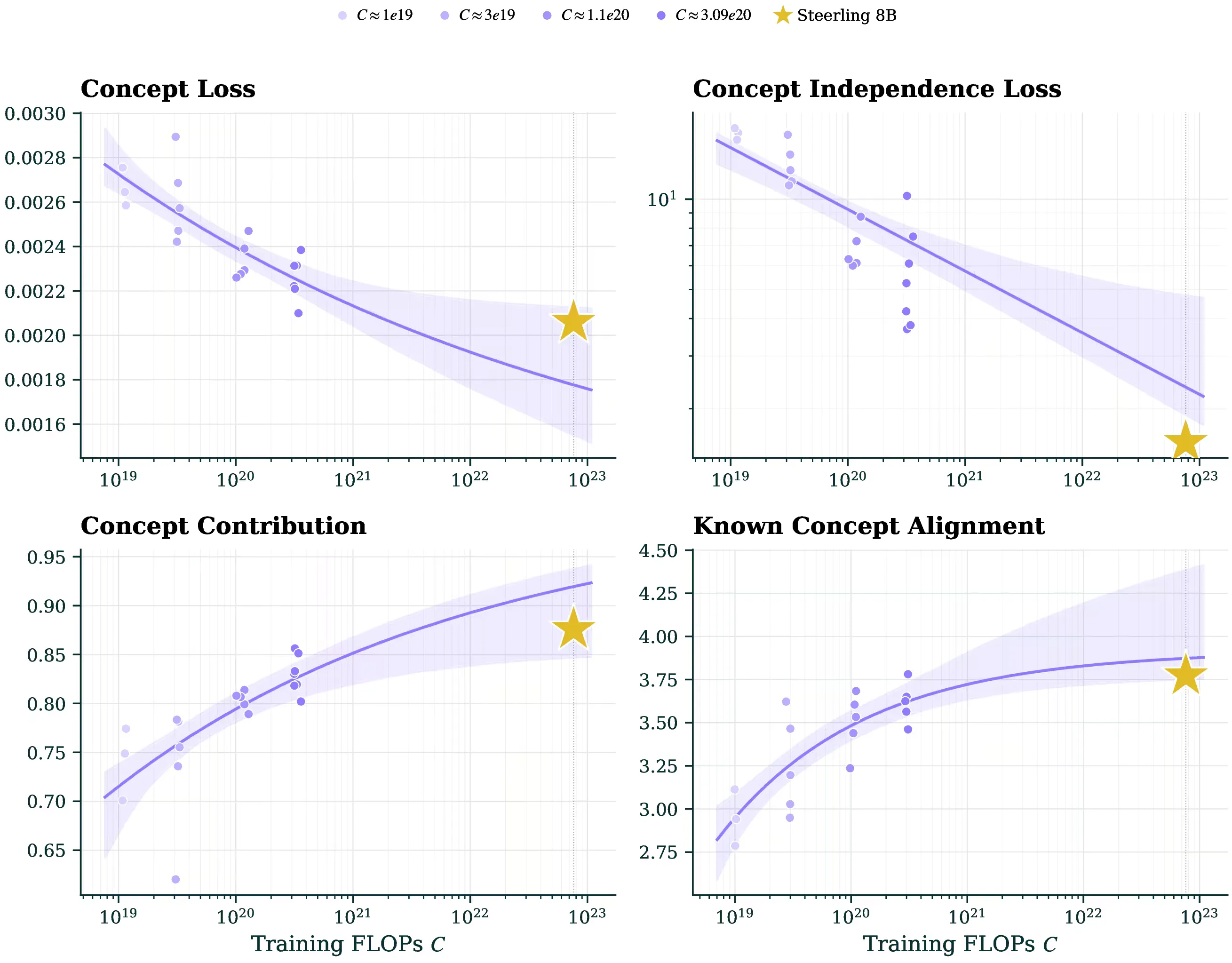
The four interpretability measures against training compute. Top row: concept detection error and concept entanglement (lower is better). Bottom row: the share of each prediction flowing through concepts, and how well concept embeddings match their human labels (higher is better). Stars: Steerling-8B, landing close to predictions made from much smaller models.
Even with the coarse scaling law, we already observe interesting insights that are counter to the prevailing narrative: we see that all the metrics improve with compute. More importantly, we now have a way to extrapolate and forecast what these properties will be as we increase compute. Below we observe the results of that extrapolation.
Three of the four properties landed close to their small-scale predictions. The fourth, Concept Independence Loss, was better than predicted.
A fine-grained scaling law
Total compute is an incomplete description of a training run. For intuition, training compute is approximately
where is the number of parameters and is the number of training tokens. In practice, one is often either data or compute constrained. We would like to cleanly tease out the effect of the model size and the training data separately on these four metrics.
To separate the effect of model size from the effect of training data, we fit each property jointly to parameters and tokens:
Now the exponents for the two components encode separate meaning: measures how quickly an interpretability property changes with model size. The second exponent, , measures how quickly it changes with training data. Each interpretability property now sweeps a surface over the parameter-token plane, where the shape of the surface encodes critical insights.
We find that the joint law explains substantially more of the differences between checkpoints than compute alone. Across the two model families, the compute-only fits obtain values between 0.49 and 0.75. Once parameters and tokens are modeled separately, this rises to between 0.62 and 0.94. Equal-compute checkpoints are not varying randomly. They differ systematically according to how the training budget was allocated.
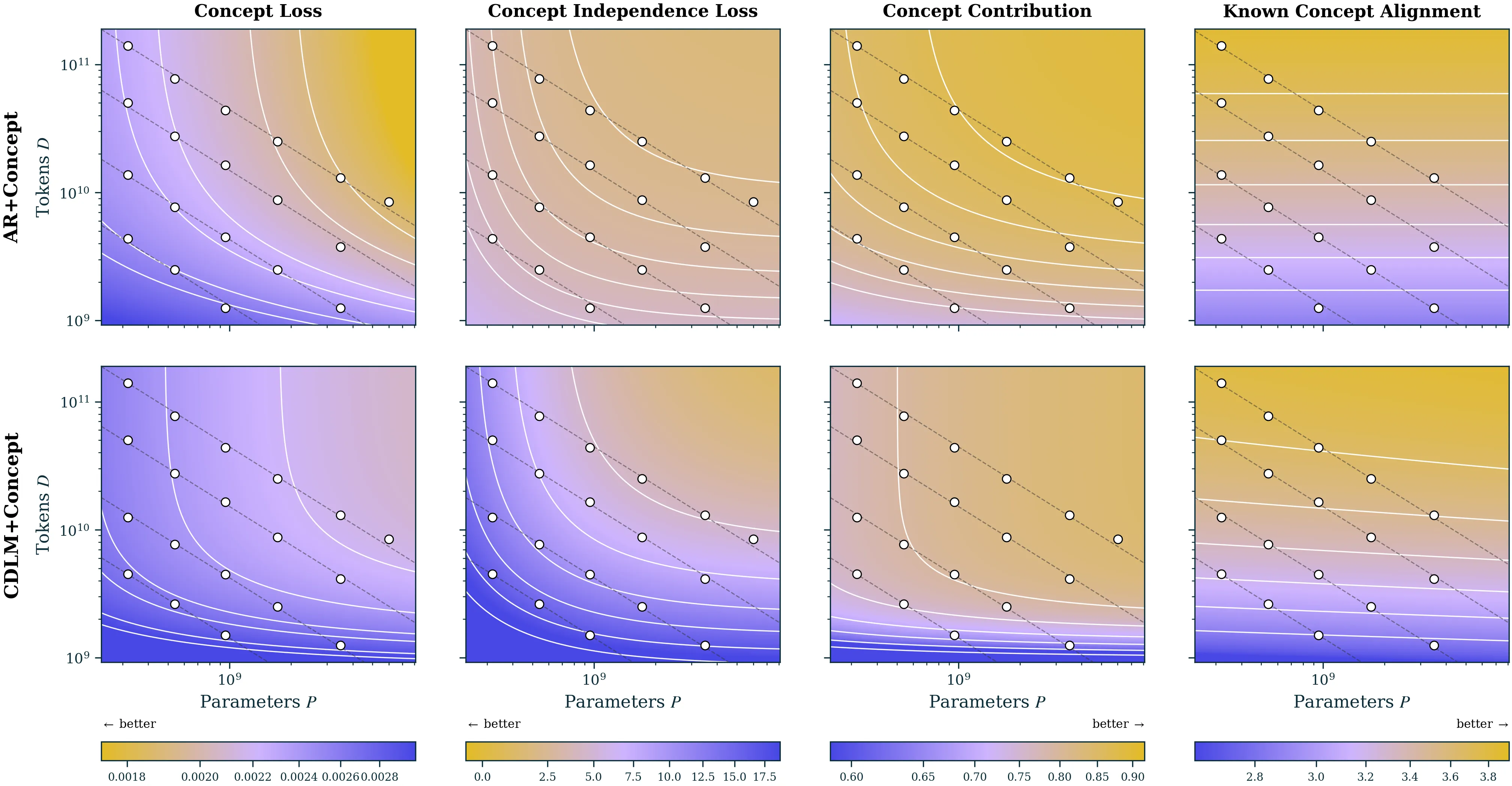
Fitted interpretability surfaces over parameters and tokens.
Gold indicates better values; each metric column shares a single color scale.
White markers: checkpoints at their trained (); dashed diagonals: IsoFLOP slice budgets.
Top row: AR+Concept; Bottom row: CDLM+Concept.
Near-vertical contours indicate parameter-driven metrics; near-horizontal, token-driven ones.
More Parameters Improves Representation Disentanglement. We find that concept detection and concept separation respond most strongly to model size. Moving horizontally across the surface, i.e. changing the number of parameters, crosses the contours more quickly than moving vertically by adding tokens. This means that a larger model trained on fewer tokens can detect the labeled concepts more accurately and maintain a cleaner division between its known and discovered representations. One possible explanation is geometric: a larger representation has more room to encode a large concept vocabulary while preserving a complementary discovered pathway.
More Training Data Improves Alignment. We find that the concept alignment metric behaves differently. In our architecture, each concept has a learned embedding that is linearly transformed into logits across the vocabulary. Consequently, we know which tokens that an embedding most promotes. We can then check the correspondence between the tokens/words a learned embedding will most promote and the name and description a human will say they should mean. Here, we find that exposure to more data makes each learned concept direction better match the meaning that a human assigned to it. Perhaps more intuitively, a possible explanation is that a larger model provides more capacity for encoding a concept while more data clarifies what the concept means.
What we can now forecast
The fine-grained scaling laws helps to elicit tradeoffs that need to be made before a large model is trained. Below we discuss its key benefits, and new affordances that it provides.
- Interpretability can be forecasted before undertaking an expensive run. As we show, a small-scale model can help estimate how a property changes with compute, and parameter–token surfaces reveal how the proposed model size and data budget will distribute this improvement.
- Compute can be allocated for the kind of interpretability requirement that is needed. Use cases that depend on independently controllable concept directions may favor more model capacity, while use cases that require concept labels to be legible to an expert may benefit more from increased training data.
- Quantitative and precise interpretability targets can be specified in training runs. A training run can now specificy plans that include thresholds such as maximum concept loss, maximum concept independence Loss, minimum concept contribution, or minimum known concept alignment scores, in addition to the usual validation-loss target.
- The marginal return from parameters and data can be estimated. The fitted surface tells us whether the next increment of compute is better spent increasing model size or data.
- Interpretable training recipes can be compared directly. When a new interpretable architecture, objective, or data mixture is proposed, it can be compared against others using these properties.
Taken together, our results provide a different scaling paradigm for powerful AI systems. Human alignment, understanding, and steerability need not be retrofitted after training. They can be specified as a requirement, optimized as part of the training process, and measured as models scale. Consequently, the opacity of today’s most capable systems is not a law of nature.