At Guide Labs we train many interpretable models at scale. Scale in itself is a challenge, and training interpretable models often comes with additional challenges, such as the need to store chunk-level concepts or document-metadata along with tokens.

Existing dataloaders forced us to choose between flexibility, reliability, and performance. We needed a dataloader that treats concepts and metadata as first-class features, shuffles and reads reliably at scale, and handles prefetching and checkpointing together.

In this article, we take you through the entire process of developing this dataloader. From the initial motivations and challenges we faced, to our design considerations, and the final implementation.

Why we built a dataloader

Implementing your own dataloader in PyTorch with torch.utils.data.DataLoader is easy if you can have all of the data in memory or can just read local files sequentially. However, this stops being feasible for large scale datasets and distributed settings. Our pre-training corpus is 1.1 trillion tokens, about 4TB of token data (assuming 32bits per token), for which we need multiple shuffled versions as we run multiple epochs. This level of scale is far beyond what torch.utils.data.DataLoader can efficiently handle.

There are existing solutions to solve this scaling challenge, such as litdata, nanotron’s TokenizedBytes or nanosets, and OLMo-core’s dataloader. Unfortunately, because all of these solutions work on either strictly token-streams or documents, none of these were sufficient for our concept-oriented model training, where we annotate token-spans in a token-stream with concepts.

Concepts: neither documents nor token-streams

Dataloaders work typically either in a token-stream mode or document mode. In a token-stream model, multiple documents are concatenated into one really large document. Each observation is then a slice from this really long document, where the slice’s size depends on the context-window. This mode is used in pre-training and mid-training, where adding padding tokens is a big waste of computation and where the context-window can change due to either debugging or long-context training.

In document mode, each observation matches exactly one document; this is how dataloading typically works. This mode is often used during post-training, where documents are multi-turn conversations, and we want the context-window to start with the special tokens used to wrap each message.

What is missing from these standard categories is how to associate additional data (metadata) with a span of tokens in the token-stream. This metadata could be a list of concepts related to a chunk of tokens, or it could simply be a document ID used for traceability when debugging. We call this “stream-with-metadata”. Existing solutions don’t support this, hence we had to build it.

Our solution not only supports stream-with-metadata, it also avoids many of the typical compromises we have found in other dataloaders when training at scale. Therefore, we also implemented support for the typical documents and token-stream modes, such we can benefit from these advantages in all situations.

What makes a great dataloader at scale

The need for concepts was on its own enough motivation for us to build a new dataloader. However, before diving into how we built it, it’s worth reflecting on the hard lessons we and others have learned, when it comes to dataloading at scale.

HuggingfaceTB’s The Smol Training Playbook provides an excellent narrative and explanation of the challenge of training at scale, and generally matches our experiences. We are here summarizing those experiences.

Minimize data transfer and coldstart time

• HuggingfaceTB initially used Weka, where data is kept on S3 and then transferred to a local network drive. Unused data is evicted from the local network drive and then has to be refetched later, which halves their throughput .

• As an alternative, HuggingfaceTB transferred 24TB to each node from S3, which took 1h 30min . This is critical downtime for when a node goes down and makes debugging very slow.

Our solution is to keep all the data on a network attached filesystem (we use Oracle’s File Storage Service), and designed the dataloader such that each rank’s process only loads the data it needs at that specific time. This avoids slow coldstart and avoids saturating the bandwidth with unused data.

Use constant-time O(1) reads

• HuggingfaceTB experienced large drop spikes in throughput, due to internal indexes in nanosets, which grow unboundedly . They switched to TokenizedBytes, which didn’t have this issue.

Our solution is to build our indices and entire read pipeline, such that loading one observation takes the same time as loading any other observation.

Use perfect uniform shuffles without replacement

• After HuggingfaceTB switched to TokenizedBytes they experienced a more noisy loss curve, because each observation in a batch would come from the same document . They solved this by pre-shuffling the dataset offline and then holding separate copies for each epoch.
• Early on in our research phase, we developed a dataloader that split our dataset into shards (collections of documents, similar to litdata), where shuffling was done within each shard. However, training with this dataloader resulted in noisy loss curves because rare concepts weren’t present across all shards.

Our solution is to design a dataloader that allows us to sample without replacement (i.e. shuffling) across the entire dataset. Doing this while also satisfying constant-time reads and avoiding slow coldstarts was a challenge. However, it meant we don’t need to store multiple differently shuffled versions of the same dataset.

Design for testability in distributed settings

• Early on, we used litdata for our post-training experiments. However, we discovered that it would truncate observations after 1 epoch when used in a multi-node setting.

Testing in distributed settings is difficult and time-consuming, as it requires an elaborate CI system that provides distributed setting and all the communication slows down testing which in practice reduces the amount of tests that can reasonably be done.

Our solution is to design a dataloader where there is never any communication between ranks, besides just knowing the rank-index, total number of ranks, and the initial. This way we can easily test if the dataloader loads the intended data when running in a distributed system, without actually needing a distributed system.

Consider prefetching and accurate checkpoints simultaneously

Training an 8B language model takes considerable computational resources and hardware failures at scale are unavoidable. Therefore, when hardware failure eventually causes a crash, it’s important to be able to resume training from the exact point that a checkpoint was saved. This does not only include the weights but also the dataloader’s exact position in the dataset, such that data is neither skipped nor duplicated.

Another consideration is prefetching. Reading data from the local disk or network attached storage to pinned memory takes time. To prevent data reading from halting training, observations should be prepared in advance in the background; this background processing is called prefetching.

• Using litdata in our post-training experiments, we discovered that checkpoints were not always exact and would often shift by one batch. From our debugging, we hypothesize that this issue is because litdata saves the position after data has been prefetched, meaning checkpoints are saved as if the prefetched data has already been used.
• OLMo-core implements its own dataloader, which does accurate checkpointing but doesn’t do any prefetching.

These examples emphasize the importance of designing the checkpointing and prefetching together. A somewhat counterintuitive insight, as these two tasks are often considered independently. Our solution designs these two aspects to work together seamlessly.

Our functional and performance requirements

After using different dataloaders ourselves and reading others’ experiences, it was clear that there wasn’t anything which met all our requirements. The dataloaders we found all had some limitations, and if we had tried to maneuver in our concept annotations, those limitations would only have gotten worse.

Considering all this, we therefore made the call to make our own dataloader designed for large scale training and streaming-with-metadata. This dataloader should satisfy our entire wishlist of functional and performance requirements.

Designing and building a dataloader for scale

When starting out with designing any complex piece of software, it’s useful to first think about what the functional requirements are and how they inform the solution.

• Because our requirements include online and uniform shuffling of the whole dataset multiple times, without keeping multiple copies of the same dataset, the data storage should be random addressable.
• Because we need precise checkpoints and data should be distributed without communication, the observations should be representable by a sequential numerical index.

These two observations work quite well together. Essentially, we can think of the dataset as a list (dataset) that isn’t loaded into memory, and then select elements from it using a plain list-index (e.g. dataset[i] = {token_ids: [1,2,7,5], concepts: [14, 25]}. How we achieve this is covered in Data layouts for zero-overhead and zero-copy reads. For now, we will just assume it’s possible.

We will also assume it’s possible to map a sequential index (e.g. 2 from range(1000)) to a seeded and shuffled position (e.g. shuffle(2, seed) = 593), such that no two index maps to the same position, given the same seed, and we will assume this can be done on-the-fly in constant time and constant memory. How we do this is covered in Online constant-time distributed shuffling using Feistel Networks.

Zero-communication distributed dataloading

With random access (dataset[i]) and shuffle (shuffle(i, seed)) components put aside, we can focus on the high-level pipeline: how we distribute data and do checkpointing.

The central idea is that if we represent all observations as indices from 0 to len(dataset), we can distribute observations to each rank using range(rank, len, ranks) . This will skip observations by the number of ranks (ranks) on each rank and offset the starting position by the rank index itself. We can also track how many observations have been read, and offset the starting position when resuming from a checkpoint with range(start + rank, len, ranks).

With this design, the reset is just applying the shuffling to the indices, gathering the data, batching the data, and finally pinning the data. Essentially, our implementation looks like this:

from itertools import batched
from functools import partial

def make_dataloader[DataT](
  dataset: Sequence[DataT],
  collate_fn: Callable[[DataT], torch.Tensor],
  epoch: int = 0,
  checkpoint: int = 0,
  rank: int = 0,
  ranks: int = 1,
  batch_size: int = 1,
  prefetch: int = 0
):
    indices = range(checkpoint*batch_size*ranks + rank, len(dataset), ranks)
    shuffled = map(partial(shuffle, seed=epoch), indices)
    data = map(lambda i: dataset[i], shuffled)
    batches = batched(data, batch_size)
    concatted = map(collate_fn, batches)
    pinned = map(lambda batch: batch.pin_memory(), concatted)
    prefetched = prefetcher(pinned, prefetch)
    return pinned

The actual implementation is a little more complicated, because we want each part to happen in a thread such that it doesn’t block the main process. We also haven’t discussed how prefetching (prefetcher) is done, and we need to support when collate_fn outputs multiple tensors. However, these details are easily handled using torchdata.nodes. Other than this, and a couple of extra details regarding epochs and updating the checkpoint state, the flow and logic is exactly as shown.

Online constant-time distributed shuffling using Feistel Networks

As established, we need a function shuffle(i, seed) that given a seed can map any index i in the range 0 to len(dataset) to an index in that same range, while ensuring that no two indices map to the same index, i.e., it should perform random sampling without replacement, better known as shuffling.

If we just needed random sampling with replacement, the solution would be simple. We can do that with numpy.default_rng(seed).integers(0, len(dataset)). However, using this would mean that in each epoch one observation can be read multiple times or zero times, where we need each observation to be read exactly once and by only one of the ranks.

Random sampling without replacement can be done using numpy.argsort on random numbers, it’s essentially numpy.argsort(np.default_rng(seed).uniform(size=len(dataset)) . NumPy even has a built-in function for this, numpy.default_rng(seed).permutation(len(dataset)), that essentially does the same. However, both of these implementations require precomputing and storing the entire shuffle mapping for the entire dataset. With 1.1 trillion tokens and a context length of 4096 tokens, that becomes 268 million indices or approximately 1GB of indices (assuming 32-bit integers). While this is certainly feasible at this scale, it would become infeasible at even larger scales. Additionally, it takes about 1 minute to compute the shuffle map. During this time, it’s not even possible to terminate the process using Ctrl+C, which makes for a rather frustrating development experience. A good development experience is not something to underestimate, as it is essential for an efficient development cycle. Still knowing this was an option at our current scale, was what gave us the confidence to choose the index-based distribution strategy discussed in Zero-communication distributed dataloading.

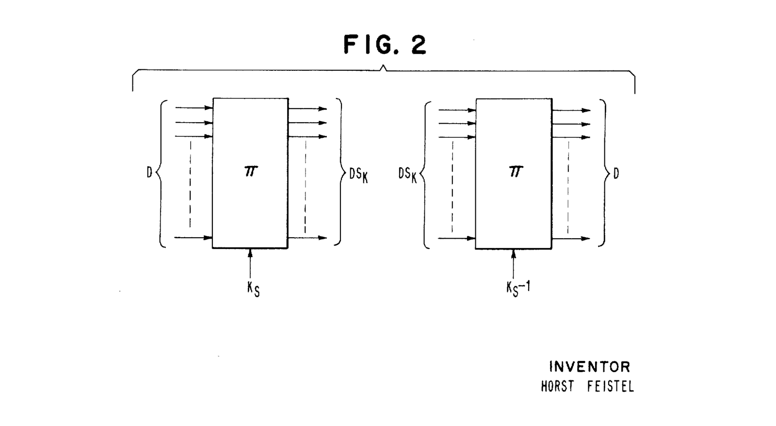
However, it turns out there is a much better solution, which allows us to compute the shuffle map on demand in O(1) memory and time rather than precomputing it, which eliminates both the memory and precompute issues. That solution is called a Feistel Network .

The general idea in a Feistel Network is that if a function $y=f(x)$ has an inverse function $g(y)$ such that $g(f(x)) = x$, then $f(x)$ is injective, meaning that every input $x$ maps to a different $y$ (otherwise it cannot be consistently inverted).

A Feistel Network provides such an invertible function, making it injective. Additionally, because the $x$ and $y$ domain is the same, $f(x)$ is also bijective. Meaning, each $x$ maps to one unique $y$ and doesn’t skip any indices.

Finally, a Feistel network can have the cryptographic property that the mapping is pseudorandom, given a fixed seed. A pseudorandom bijective mapping is exactly what shuffling is, and is why a Feistel Network is a great tool for doing random shuffling without precomputing a mapping. As a real world example, it is infamously used to distribute credit/debit card numbers in a seemingly random order, without risking that two customers end up with the same credit/debit card numbers.

Understanding how a Feistel Network works when the range is even-bit integers ($0 \le x < 2^{2\mathbb{N}}$) isn’t too complicated. It becomes more complicated once we consider any positive integer range, which we have. Fortunately, this is a solved problem with a nearly identical idea; and there is a Python implementation called gfc which implements it, hence we will skip that detail here and focus on the even-bit integer range.

How a Feistel Network works

First, some basic definitions:

• The set $\mathbb{B}_n$ contains all the positive integers of $n$ bits, i.e. $\mathbb{B}_n = \{0, 1, \cdots, 2^{n} - 1\}$.
• Consider an input $x \in \mathbb{B}_{2n}$.
• Define a “round-function” $h = F(v, k)$ that takes a value $v \in \mathbb{B}_n$ and does a pseudorandom mapping to the same domain $h \in \mathbb{B}_n$ using a key $k$. Note that this function does not need to be invertible or injective. Often, a hashing function is used (gfc uses Speck).

Then, to compute the Feistel Network:

• Split $x$ into two halves, a left ($L_0 \in \mathbb{B}_n$) and right side ($R_0 \in \mathbb{B}_n$), i.e. its upper and lower bits.
• Then apply the round function on the right bits and XOR it with the left bits. This generates a new set of left and right bits, which are then swapped. $L_1 = R_0, R_1=L_0 \oplus F(R_0, k_1)$.

This continues for a few more rounds. The more rounds, the more uniform a shuffle one gets. 5 rounds are plenty to get a really good shuffle for a non-cryptographic setting. 8-16 rounds are typically used in a cryptographic setting.

The magic in the Feistel network is that given any round function, even if it’s pseudorandom and non-invertible, the Feistel network itself is still invertible, which is what gives it the bijective property and makes it a great solution for shuffling.

That is it, a Feistel network just involves applying xor operations and round-functions in a sequence. For shuffling, we don’t even need to run the inverted Feistel network; it’s enough to know that because inversion is possible and the output and input domain is the same, a Feistel network is bijective. The proof for pseudo-randomness is more complicated, but intuitively it’s because we use a pseudorandom round-function.

Data layouts for zero-overhead and zero-copy reads

Now that we have established how to do shuffle(i, seed), the final piece of the puzzle is how to implement dataset[i] . There are two criteria here when reading dataset[i]:

• We should only read the bytes corresponding to that observation. If we have to read more, that’s wasted resources.
• Our format should “speak NumPy” natively. If we have to decode our storage format into numpy, then we have to copy data and compute the reformatting. That is overhead we would like to avoid. Once the format is NumPy, we can use e.g. torch.from_numpy() to make it PyTorch compatible without copying data.

On the other hand, because we are optimizing for an HPC system, there are some affordances we can make. Specifically distributed file systems, like Lustre or Oracle’s File Storage Service, are often optimized for random reads, as long as the reads are not too small (e.g 4KB for FSS ). Additionally, the bandwidth and disk availability is often great enough to not require compression.

Structured NumPy arrays

It’s often wise to start with the most constraining requirement when considering solutions. In this case, “speak NumPy” is by far the hardest constraint. Therefore, before describing the actual data format, it’s worth first understanding numpy-structured-arrays and its binary format.

The most well-known use of NumPy dtypes is probably np.array([1,2,3], dtype=np.int16). Here NumPy allocates 2 bytes (16 bits) to each integer (we are glossing over endian-ordering here), and then stores them in sequence. Such that if you ask for the value at index i, it can calculate the data start position as 2 * i and then read the next 2 bytes. However, what about more complex data structures, what if we wanted to store pairs of integers but one is 16-bit, and the other is 32-bits (for example tokens and per-token concepts). Well, NumPy has an answer for this called structured arrays.

NumPy structured arrays allows us to define our own dtype:

concept_pair_dtype = np.dtype([
    ('token', np.uint32),
    ('concept', np.uint16)
])
array = np.array([(151, 1), (213, 6), (726, 3)],
                 dtype=concept_pair_dtype)
print(array[0]['token']) # 151

This works even for more complex structures, like nested structures or fixed-sized matrices, as long as the amount of bytes stored in each structured element remains fixed. NumPy even has a dtype.itemsize API for getting the number of bytes used (e.g. concept_pair.itemsize == 6). This means that for basic vectors of structured elements, we can compute the start position as index * dtype.itemsize and read dtype.itemsize bytes. Or if we wish to read 4096 consecutive elements (e.g. tokens and token-wise concepts), we can read 4096 * dtype.itemsize bytes.

Operating systems have a specific API for this, which is generally called seek .

with open('stream.bin', 'rb') as fp:
    fp.seek(index * dtype.itemsize)
    data = fp.read(length * dtype.itemsize)

To then convert the data to a structured NumPy array, we can use np.frombuffer(data, dtype=dtype). During writing to convert from array to bytes, we can use array.tobytes() there are some extra details regarding endianness, strides, and C/F ordering, which we are skipping here. However, NumPy supports all these aspects, so it’s not a problem. .

Metadata on token-spans

Using structured NumPy arrays gives a neat solution to storing and loading token-streams and extra fixed-sized token-aligned metadata. However, what happens when we want to attach metadata to a token span (e.g. concepts for a chunk of tokens or a document id) and the size of the metadata isn’t fixed? How do we know where to read from, and how do we know what metadata relates to each token?

Relating metadata to each token is fairly straightforward; we will simply give each metadata a sequential id and store it as a field in the token-stream’s structured dtype. For example, np.dtype([('token', np.uint32), ('metadata_id', np.uint32)]). If multiple tokens have the same metadata-id, the same metadata belongs to all of those tokens.

To then store the actual metadata, we will use two additional files, an index file and a data file. The data file simply stores the serialized metadata sequentially. To serialize the metadata, one could use pickle.dumps for arbitrary documents or array.tobytes() for NumPy arrays. In our implementation, we leave the serialization and deserialization entirely user-defined, such that users can choose the format themselves pickle.dumps is a fairly inefficient storage format and blocks the GIL when loading data, so using NumPy arrays is often preferred. .

Each serialization then generates a varying number of bytes, and each serialization is then stored next to each other on disk. An index file is then used to note the start position of each serialized metadata. This index file is just another NumPy array, so we can look up the sequential metadata ID in this index array, to then get the serialized metadata’s read position.

metadata_id_dtype = np.dtype(np.uint64)
with open('metadata.index', 'rb') as fp:
  fp.seek(index * metadata_id_dtype.itemsize)
  # read two elements from array
  indexdata = fp.read(2 * metadata_id_dtype.itemsize)
  start, end = np.frombuffer(indexdata, dtype=metadata_id_dtype)
with open('metadata.bin', 'rb') as fp:
	fp.seek(start)
	metadata = deserialize(fp.read(end - start))

Parallel writing using data sharding

If it was sufficient to just write all the data sequentially, the above data format is all we would need. However, preprocessing and writing trillions of tokens takes time, so ideally we would like to be able to do it in parallel. Additionally, large datasets are often composed of subsets from different sources, so there is a benefit in being able to combine data without having to re-encode everything.

The solution to this is to use sharding, where arrays are split into multiple files. This allows us to write each shard independently (e.g. in parallel), and then later treat all shards as one big array. In many other dataloaders, sharding is also used for data-transfer and shuffling, such that shards are distributed to each node and then the shard is shuffled locally. However, that is not the case for our dataloader. Entire shards are not transferred, only the data for the requested observation, and the shuffling is global and has no connection with sharding. During reading, our dataloader provides no functional difference between using shards and not using shards.

To know which shard to read from, we simply need to know the size of all token-stream shards. The size is just metadata (os.path.getsize in Python) and doesn’t require reading any of the files’ content. It does take a bit of time at startup, but compared to transferring entire shards or shuffling large arrays, it’s nothing. Once we know the size of each shard, we can compute the cumulative sum and use binary search to get the shard index.

# [124MB, 12MB, 51MB]
file_sizes = [124_000_000, 12_000_000, 51_000_000]
# [124_000_000, 136_000_000, 187_000_000]
lookup_index = np.cumsum(file_sizes)
shard = np.searchsorted(lookup_index, index * dtype.itemsize, side='right')

For our metadata, we then simply make the metadata-ids shard-local. So once we know the stream data’s shard, we also know the metadata’s shard. This also means we can get away with using a uint32 datatype for the metadata ID. That supports 4 million metadata-documents, which is not enough for the entire dataset but is enough for each shard. The alternative would be to use uint64 to store the global metadata-document index. However, as a copy of this id needs to co-exist for every token, using uint64 rather than uint32 increases the storage size of 1 trillion tokens from 8TB to 12TB. So, using local metadata IDs and limiting each shard to 4 million metadata, we can save a lot of storage, which also saves bandwidth.

As a final detail, some observations may require us to read from two files (or more if the shards are really small or the context-window is very large). However, we are able to precompute exactly which files to read from and how many bytes, so we can do multiple reads in parallel. We have an async-reader which does exactly this. However, our current PyTorch dataloader uses a sync-reader which reads one file at a time, as synchronous code works best with torchdata.nodes. But in practice, it’s inconsequential as there are at most two files and the data is prefetched.

Just stream-data and just document-data

With the metadata IDs in the token-streams and the index and serialized-data file, this storage format is able to accommodate our token-concept data structures as well as our performance criteria.

Of course, there are cases when all of this complexity isn’t needed. For example, if a user just wants a token-stream or if a user just wants document-data (no concatenation). Our format is able to accommodate these simpler variations. When using just token-stream, we just remove the metadata ID from the structured NumPy array and avoid creating the metadata files. In the document-data case, we use the metadata ID for the document index, and use the size of the index-files to get the number of documents per shard and thus compute the shard-index (again using binary-search on the cumulative sum).

From theory to practice: GIL-free index calculations, combined syscalls, and POSIX’s pread

Online sampling algorithms and NumPy’s efficient data formats are unfortunately not enough to get peak performance. The implementation details also matter a lot. For example, python itself is slow and doing many tiny read operations is also slow. Optimizing these aspects improves throughput by more than 1000 times, and is what makes the difference between a theoretically solid implementation and a practical implementation.

GIL-free index calculations with Numba JIT

When reading the stream data, for example 4096 tokens, we need to process the metadata IDs to understand which metadata documents to read and which tokens they correspond to. This is further complicated by reading multiple shards. We refer to this as index calculations. Overall, index calculations are a lot of loops and checks, something which Python is very slow at, and a slow dataloader blocks the model training.

Normally, this would be solved by using multiprocessing. However, multiprocessing is also slow because it requires serializing and copying data and sending it over an IPC (inter-process communication) channel. As we already established, serializing, copying data, and deserializing is an overhead. To avoid this overhead, we use threads, as threads allow us to share memory. However, threads in Python have the disadvantage that only one python-statement can run at the same time, due to the GIL (global interpreter lock). That means that even though the index calculations happen in a different thread than the main training loop, it will still slow down training. However, there is a loophole. The GIL is only relevant for python-statement, or more precisely, when the interpreter is involved. For non-python native code, we can free the GIL to run the training loop rather than doing index calculations. To do this, we use Numba, a tool for compiling Python and NumPy to native code. Compiling to native code speeds up computations massively. But importantly, Numba also has a no-GIL option, which ensures that the calculations run free of the GIL.

To get Numba to understand our data structures, for example, the stride and positions of each stream-file read request, we found it to be most performant to again use NumPy’s structured-arrays, as Numba has built-in support for these. However, this time they are used as datastructures for the runtime index calculations, not the data itself. When doing all of these optimizations, the code does end up looking a bit funky. However, once you get used to it, it’s fairly straightforward.

from collections.abc import Sequence

import numpy as np
from numba import njit, types, from_dtype, int64, int32

type Vector[DType: np.generic] = np.ndarray[tuple[int], np.dtype[DType]]

stream_req_dtype = np.dtype([
    ('shard', np.int64),
    ('global_offset', np.int64),
    ('shard_offset', np.int64),
    ('length', np.int64)
], align=True)

metadata_req_dtype = np.dtype([
    ('shard', np.int64),
    ('shard_index', np.int32),
], align=True)

@njit((int64, types.Array(from_dtype(stream_req_dtype), 1, 'C'), int32[:]), nogil=True)
def compute_metadata_requests_and_index(
    global_length: int,
    stream_req_list: Vector[np.void],
    metadata_ids: Vector[np.int32]
) -> tuple[Vector[np.void], Vector[np.int32]]:
    # data accumulation across all shards
    metadata_req = np.empty(global_length, dtype=metadata_req_dtype)
    metadata_local_indexes = np.empty(global_length, dtype=np.int32)

    # retrieve out-of-band map
    curr_meta_local_index = int32(-1)
    curr_meta_index_offset = int32(0)
    local_meta_i = int32(0)
    for stream_req in stream_req_list:
        prev_shard_meta_global_index = int32(-1)
        for _ in range(stream_req['length']):
            shard_meta_index_global = metadata_ids[curr_meta_index_offset] # type: ignore

            # detected new out-of-band part, so issue request
            if shard_meta_index_global != prev_shard_meta_global_index:
                curr_meta_local_index += int32(1) # type: ignore
                metadata_req[curr_meta_local_index]['shard'] = stream_req['shard']  # type: ignore
                metadata_req[curr_meta_local_index]['shard_index'] = shard_meta_index_global  # type: ignore

            metadata_local_indexes[local_meta_i] = curr_meta_local_index  # type: ignore
            local_meta_i += int32(1)  # type: ignore
            curr_meta_index_offset += int32(1)  # type: ignore
            prev_shard_meta_global_index = shard_meta_index_global  # type: ignore

    return (metadata_req[:(curr_meta_local_index+1)], metadata_local_indexes) # type: ignore

Combining reads and syscalls

In addition to slow index calculations, the other performance killer is doing many small reads, as each read needs to communicate with the operating system (syscall), which is slow. Each read also needs to request from the networked file system, which is also slow. The token-stream reads are usually fine, as 4096 tokens is 32KB, which is a reasonable size for a parallel I/O networked filesystem. However, the metadata are much worse. The index lookup is just 16 bytes, and the metadata themselves are typically 160 bytes in our case. Those reads are too tiny to be performant.

However, we can drastically optimize away these small reads. Because the metadata IDs are consecutive, we can usually combine all the metadata lookups from 4096 tokens into just one index-read and one data-read. Simply take the smallest and largest metadata ID from the 4096 tokens, and read that entire part. This will provide all of the data positions for the metadata. Then take the first and last data-positions, and read all of the metadata content in between. Using Python’s memoryview, we can then unpack the result from the combined read-instruction into multiple buffers without copying the data. The unpack code looks like this:

def _unpack_data(unpack_info: Vector[np.void],
                 datas: Sequence[bytearray]) -> Sequence[memoryview]:
    data_views = [memoryview(data) for data in datas]
    return [
        data_views[request][start:end]
        for request, start, end in zip(unpack_info['request'].tolist(),
                                       unpack_info['start'].tolist(),
                                       unpack_info['end'].tolist(),
                                       strict=True)
    ]

POSIX’s preads and other small tricks

Another frequent syscall we can remove is the seek operation. POSIX systems (e.g. Mac and Linux) have a feature that combines the seek and read, called pread. Its API is data = os.pread(fd, length, offset) .

Another trick we found is that PyTorch expects writeable data. However, fp.read and os.pread gives read-only buffers. The typical solution is to copy the read-only buffer into a writable buffer. However, there is a better way. Because we know exactly how much data to read, we can preallocate a writable buffer and read directly into this writable buffer using os.preadv. The code looks like this:

def read(self, offset: int, size: int) -> bytearray:
    content = bytearray(size)
    bytesread = os.preadv(self.fd, (content, ), offset)
    assert bytesread == size
    return content

There are many more small tricks, which we didn’t spend time on benchmarking. For example, on Linux, we can instruct the operating system that the reads are entirely random, such it doesn’t try to read ahead and cache the following data (typically smart for sequential reads, but not for random reads). In Python, one can use os.posix_fadvise(fd, 0, 0, os.POSIX_FADV_RANDOM).

Conclusion

It’s a fairly big endeavor to make a dataloader for training at scale, as there are many technical and practical considerations and ensuring everything works requires extensive testing. However, it can be worthwhile. Not only is it important for training speed, but global shuffling, consistent checkpoints, and reliable behavior is important for the model’s accuracy as well.

At Guide Labs we have used this dataloader extensively. It has been used for pre, mid, and post-training of Steerling, an 8B interpretable language model where we incorporate concept annotations during training. It has been used to train PRISM, an interpretable language model for identifying relevant training data. Training either of these models without a highly flexible and efficient dataloader would have been impossible.

To help others achieve the same benefits, we plan on open-sourcing the dataloader in the coming months, so sign up to our mailing list to get notified when it will be released.

While we haven’t used the dataloader to train on images, video, and multi-modal data yet, its general design should allow for such use cases and we look forward to see how people will use it.